この記事では、Amazon ChronosとGridDBデータベースを使用して、電力生産のタイムシリーズ予測モデルを構築する方法を説明します。
Kaggleから過去の電力生産データを取得し、GridDBのタイムシリーズコンテナに格納します。その後、T5アーキテクチャを基盤としたタイムシリーズモデル専用のコレクションであるAmazon Chronosを使用して、予測モデルをトレーニングします。
GridDBは、大規模なリアルタイムデータの処理に最適化された堅牢なNoSQLデータベースです。高度なインメモリ処理と時系列データ管理機能により、ビッグデータやIoTアプリケーションに最適です。
GridDBのリアルタイムデータ処理機能とChronosの最先端予測手法は、時系列予測アプリケーションにおいて強力な組み合わせとなります。
事前準備
この記事のコードを実行するには、以下のライブラリをインストールする必要があります。
- GridDB Cクライアント
- GridDB Pythonクライアント
これらのクライアントのインストール手順は、以下のリンクから確認できます。 GridDB Python パッケージ インデックス.
Amazon Chronos、Numpy、Pandas、およびMatplotlibのライブラリをインストールする必要があります。
以下のスクリプトは、コードを実行するために必要なライブラリをインストールし、インポートするのを助けます。
%pip install git+https://github.com/amazon-science/chronos-forecasting.git
%pip install matplotlib seaborn numpy pandas scikit-learn
import matplotlib.pyplot as plt
from matplotlib.dates import DateFormatter
import seaborn as sns
import numpy as np
import pandas as pd
import torch
from chronos import ChronosPipeline
import griddb_python as griddb
from sklearn.metrics import mean_absolute_errorグリッドDBに時系列データを挿入する
最初のステップは、予測対象の時系列データをグリッドDBに挿入することです。このセクションでは、その手順を説明します。
Kaggleから電力生産データをダウンロードしてインポートする
私たちは、Kaggleからの電力生産データセットを使用して、将来の電力生産需要を予測します。
以下のスクリプトは、データセットを含むCSVファイルをpandas DataFrameにインポートします。
dataset = pd.read_csv("Electric_Production.csv")
dataset.head(10)
出力:
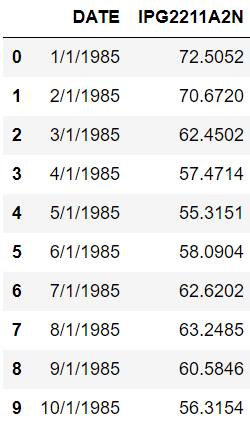
データセットは、1985年1月1日から2018年1月1日までの月次電力生産量から構成されています。
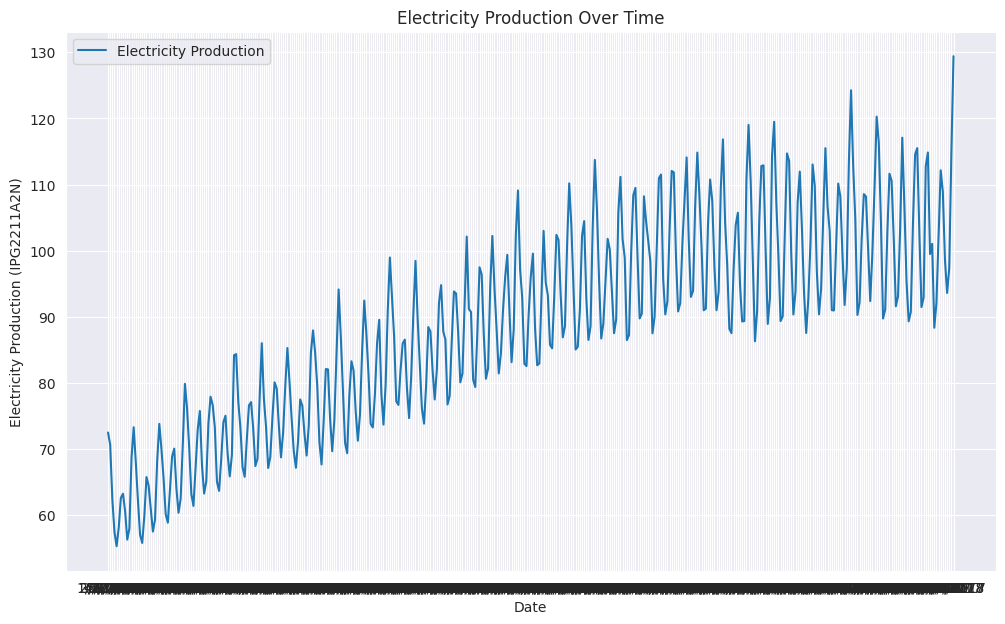
線グラフを作成することで、電力生産量が年の月によって大きく異なることが確認できます。
# Create the line plot
sns.set_style("darkgrid")
plt.figure(figsize=(12, 7))
sns.lineplot(data=dataset, x='DATE', y='IPG2211A2N', label='Electricity Production')
plt.xlabel('Date')
plt.ylabel('Electricity Production (IPG2211A2N)')
plt.title('Electricity Production Over Time')
plt.legend()

plt.show()
出力:
データセットが用意できたら、このデータをGridDBに挿入できます。
GridDBへの接続
GridDBに接続するには、StoreFactoryクラスのオブジェクトを作成する必要があります。次に、ストアファクトリオブジェクトのget_store()メソッドを呼び出し、DBホスト名、クラスター名、ユーザー名、パスワードを引数として渡します。
接続が正常に確立されたかどうかを確認するには、get_container()メソッドを呼び出し、任意のコンテナ名を引数として渡します。以下の出力が表示されれば、接続は成功しています。
# GridDB connection details
DB_HOST = "127.0.0.1:10001"
DB_CLUSTER = "myCluster"
DB_USER = "admin"
DB_PASS = "admin"

# creating a connection

factory = griddb.StoreFactory.get_instance()

try:
    gridstore = factory.get_store(
        notification_member = DB_HOST,
        cluster_name = DB_CLUSTER,
        username = DB_USER,
        password = DB_PASS
    )

    container1 = gridstore.get_container("container1")
    if container1 == None:
        print("Container does not exist")
    print("Successfully connected to GridDB")

except griddb.GSException as e:
    for i in range(e.get_error_stack_size()):
        print("[", i, "]")
        print(e.get_error_code(i))
        print(e.get_location(i))
        print(e.get_message(i))
出力:
Container does not exist
Successfully connected to GridDB
グリッドDBに電力生産データ用のコンテナを作成する
グリッドDBはデータコンテナを格納します。コンテナを作成するには、コンテナ名と列の情報が必要です。
コンテナには任意の名前を付けることができます。ただし、コンテナ情報は、各ネストされたリストが列名と列タイプを含むリストのリストで構成される必要があります。
例えば、以下のスクリプトでは2つの列があります:TimeStamp(列タイプ griddb.Type.TIMESTAP)と Production(列タイプ griddb.Type.DOUBLE)。
次に、ContainerInfo クラスのオブジェクトを作成し、コンテナ名と列情報を ContainerInfo クラスのコンストラクタに渡しします。
最後に、put_container() メソッドを呼び出し、ContainerInfo クラスのオブジェクトを引数として渡すことで、GridDB にコンテナを作成します。
dataset['DATE'] = pd.to_datetime(dataset['DATE'])


container_name = "Electricity_Production"
column_info = [
    ["Timestamp", griddb.Type.TIMESTAMP],
    ["Production", griddb.Type.DOUBLE]
]
container_info = griddb.ContainerInfo(container_name, column_info, griddb.ContainerType.TIME_SERIES)

# Creating Container
try:
    gridstore.put_container(container_info)
    container = gridstore.get_container(container_name)
    if container is None:
        print(f"Failed to create container: {container_name}")
    else:
        print(f"Successfully created container: {container_name}")

except griddb.GSException as e:
    print(f"Error creating or retrieving container {container_name}:")
    for i in range(e.get_error_stack_size()):
        print(f"[{i}]")
        print(f"Error code: {e.get_error_code(i)}")
        print(f"Location: {e.get_location(i)}")
        print(f"Message: {e.get_message(i)}")
出力
Successfully created container: Electricity_Production作成したコンテナは、get_container() メソッドを使用して取得できます。
次に、作成したコンテナにデータセットを格納します。
電力生産データをGridDBコンテナに挿入
GridDBコンテナにデータを挿入するには、データセットのすべての行を反復処理し、コンテナオブジェクトのput()メソッドを呼び出し、DATEとIPG2211A2N列の値をメソッドに渡しします。
try:
    for index, row in dataset.iterrows():
        container.put([row['DATE'].to_pydatetime(), row['IPG2211A2N']])
    print(f"Successfully inserted {len(dataset)} rows of data into {container_name}")

except griddb.GSException as e:
    print(f"Error inserting data into container {container_name}:")
    for i in range(e.get_error_stack_size()):
        print(f"[{i}]")
        print(f"Error code: {e.get_error_code(i)}")
        print(f"Location: {e.get_location(i)}")
        print(f"Message: {e.get_message(i)}")
出力
Successfully inserted 397 rows of data into Electricity_Production電気発電データをGridDBに正常に挿入しました。次のステップは、AmazonのChronosモデルを使用して電気発電量を予測することです。
AmazonのChronos時系列モデルを使用した電気発電量の予測
Amazon Chronosは、事前トレーニング済みの言語モデル群です。これらのモデルは、時系列データに対応するように適応されたT5(Text-to-Text Transfer Transformer)アーキテクチャを基盤としています。
GridDBからのデータ取得
電力生産の予測を行うため、まずGridDBに保存したデータを取得する必要があります。これには、取得したいコンテナ名を引数に指定してget_container()メソッドを使用します。
コンテナの query() メソッドを使用して SELECT * クエリを実行します。次に、fetch() メソッドを呼び出してデータセットオブジェクトを取得します。最後に、fetch_rows() メソッドを呼び出してデータセットを pandas DataFrame に格納します。
def retrieve_data_from_griddb(container_name):
try:
stock_data_container = gridstore.get_container(container_name)
# Query all data from the container
query = stock_data_container.query("select *")
rs = query.fetch() # Adjust the number based on your data size
data = rs.fetch_rows()
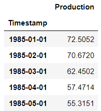
data .set_index("Timestamp", inplace=True)
return data
except griddb.GSException as e:
print(f"Error retrieving data from GridDB: {e.get_message()}")
return None
electric_production_data = retrieve_data_from_griddb("Electricity_Production")
electric_production_data.head()出力:
Amazon Chronos モデルを用いた電力生産の予測
Amazon Chronos モデルは Hugging Faceで無料で利用可能です。推論を行うためには、GitHub.からモデルをインストールするだけです。
データセットをトレーニングセットとテストセットに分割します。次に、Amazon Chronosモデルを使用して、テストセットの月ごとの電力生産量を予測します。最後に、予測した電力生産量と実際の生産量を比較して、モデルの性能を評価します。
以下のスクリプトはデータセットをトレーニングセットとテストセットに分割します。データセットには合計397件のレコードが含まれています。テスト用に最後の47件を使用します。
# Define the test size and calculate the split index
test_size = 47
split_index = len(electric_production_data) - test_size

# Check if the data length is shorter than the test size
if split_index < 0:
    train_production = pd.Series(dtype=float)
    test_production = electric_production_data['Production']
else:
    # Splitting the Production column into training and test sets
    train_production = electric_production_data['Production'].iloc[:split_index]
    test_production = electric_production_data['Production'].iloc[split_index:]

# Display the results
print("Training Set:")
print(train_production.shape)
print("\nTest Set:")
print(test_production.shape)
出力:
Training Set:
(350,)

Test Set:
(47,)次に、ChronosPipeline.from_pretrained() メソッドを使用して、事前学習済みの Chronos t5 large モデルをインポートします。
pipeline = ChronosPipeline.from_pretrained(
  "amazon/chronos-t5-large",
  device_map="cuda",
  torch_dtype=torch.bfloat16,
)Chronosモデルは、データがTorchテンソル形式で格納されていることを想定しています。以下のスクリプトは、データをTorchテンソルに変換します。次に、トレーニングデータ(コンテキスト)に基づいて、次の47ヶ月分の電力生産を予測するために、pipeline.predict()メソッドを使用します。
予測結果を3つの四分位数(0.1、0.5、0.9)に分割します。
context = torch.tensor(train_production)
prediction_length = test_size
forecast = pipeline.predict(context, prediction_length)
low, median, high = np.quantile(forecast[0].numpy(), [0.1, 0.5, 0.9], axis=0)
次に、モデルの性能を評価します。
モデルの性能評価
予測値の中央値をテスト値に対してプロットします。そのため、予測値を含むpandas DataFrameを作成します。
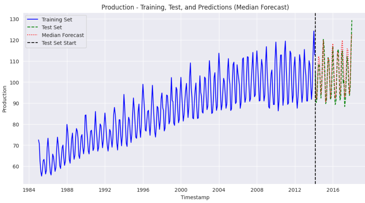
以下のスクリプトは、トレーニングセット、テストセット、および予測値をプロットします。
test_production.index = pd.to_datetime(test_production.index)
median_forecast = pd.Series(median, index=test_production.index, name="Median Forecast")

plt.figure(figsize=(12, 6))
plt.plot(train_production.index, train_production, color='blue', label="Training Set", linestyle="-")
plt.plot(test_production.index, test_production, color='green', linestyle="--", label="Test Set")
plt.plot(median_forecast.index, median_forecast, color='red', linestyle=":", label="Median Forecast")

# Vertical line to mark the start of the test set
plt.axvline(x=test_production.index[0], color='black', linestyle="--", label="Test Set Start")

plt.xlabel("Timestamp")
plt.ylabel("Production")
plt.title("Production - Training, Test, and Predictions (Median Forecast)")
plt.legend()
plt.show()
出力:

上記の出力結果から、当社のモデルが良好な性能を示し、トレーニングデータセットの傾向を適切に捕捉できていることがわかります。予測値はテストセットの値に近接しています。
次に、テスト値のみを中央値の予測値と80%予測区間に対してプロットします。
median_forecast = pd.Series(median, index=test_production.index, name="Median Forecast")
lower_bound = pd.Series(low, index=test_production.index, name="Lower Bound")
upper_bound = pd.Series(high, index=test_production.index, name="Upper Bound")


plt.figure(figsize=(12, 6))

plt.plot(test_production.index, test_production, color='green', linestyle=":", label="Actual Production")
plt.plot(median_forecast.index, median_forecast, color='red', linestyle=":", label="Median Forecast")

# Plot the 80% prediction interval as an orange shaded area
plt.fill_between(test_production.index, lower_bound, upper_bound, color='orange', alpha=0.3, label="80% Prediction Interval")

plt.xlabel("Timestamp")
plt.ylabel("Production")
plt.title("Production - Actual vs. Forecast with 80% Prediction Interval")
plt.legend()
plt.show()
出力:
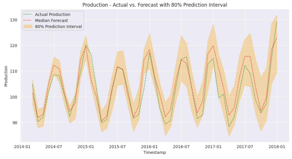
上記の出力結果から、予測値の80%区間がテストデータのほぼすべてをカバーしていることがわかります。これにより、当社のモデルが時系列データの予測において極めて高い性能を発揮していることが示されています。
最後に、予測結果の平均絶対誤差(MAE)値をプロットし、結果を定量化します。
mae = mean_absolute_error(test_production, median_forecast)

# Print results
print("Average electricity production values in the training set:", train_production.mean())
print("Mean Absolute Error (MAE):", mae)
出力:
トレーニングセットにおける平均電力生成値: 86.9775362857143 平均絶対誤差 (MAE): 3.2303302385930803
MAE値は3.23となり、平均して当社のモデルの予測値は実際のテスト値から3.23単位の誤差があり、トレーニングセットの平均電力生産量から3.4%の偏差を示しています。
結論
本記事では、GridDBとAmazon Chronosを使用した時系列予測の完全なワークフローを解説しました。GridDBへの接続方法、時系列データの挿入、Amazon Chronosモデルを訓練して電力生産を予測する手順を確認しました。結果は、季節的な傾向を正確に捉え、80%の信頼区間内で信頼性の高い予測を提供しました。
GridDBの堅牢な時系列データ管理とChronosの専門的な予測モデルを組み合わせることで、正確な時系列予測を実現するスケーラブルなソリューションが提供されます。
ブログの内容について疑問や質問がある場合は Q&A サイトである Stack Overflow に質問を投稿しましょう。 GridDB 開発者やエンジニアから速やかな回答が得られるようにするためにも "griddb" タグをつけることをお忘れなく。 https://stackoverflow.com/questions/ask?tags=griddb