迷信深い人は、自分のラッキーナンバーで勝負したほうが宝くじに当たる可能性が高いと信じているのかもしれません。自分の選んだ数字が抽選される可能性が高いと信じているのです。
もちろん、宝くじが不正に操作されていない限り、そのようなことはありません。ほとんどの人は、どの数字も、どの数字の組み合わせも、同じ可能性を持っていることに気がつくでしょう。しかし、ここが面白いところですが、すべての組み合わせが同じ期待値を持っているわけではありません。
私たちの考えはこうです。迷信深い人もいますし、人間はランダムに数字を選ぶのが苦手なので、ギャンブラーが他の数字よりずっと頻繁にプレイする数字があります。他の人がプレイする可能性が最も低い数字をプレイできれば、実際に勝った場合、より少ない人数でポットを分けられるので、より多くのお金を獲得できることが期待できるのです。
ですから、長期的に見れば、より多くのお金を稼ぐことができる数字があることは事実です。より多くのお金を稼ぐというのは、平均的な宝くじプレイヤーよりも遅い速度でお金を失うという意味で、それでもお金を失うことに変わりはありません。
ソースコードの全文はこちらでご覧いただけます。https://github.com/retowyss/swisslos-r-griddb/
$ git clone https://github.com/retowyss/swisslos-r-griddb.git データの概要と分析ツール
スイスの国営宝くじ「Swisslos」の約7年分の抽選結果(n = 720, start = 2013-01-12, end = 2019-12-04)を、統計プログラミング言語Rを用いて分析し、データの保存にはGridDBを使用しています。
# Required packages RJDBC and tidyverse
# griddb is the connection object to our GridDB

drv <- JDBC(
  driverClass = "com.toshiba.mwcloud.gs.sql.Driver",
  # Point this to your gridstore jar
  classPath = "/jdbc/bin/gridstore-jdbc.jar"
)

# IP and port depend on your setup
griddb <- dbConnect(
  drv,
  "jdbc:gs://172.20.0.42:20001/dockerGridDB/public",
  "admin",
  "admin"
)

# vectorized insert function
dbInsertTable <- function(conn, name, df, append = TRUE) {
  for (i in seq_len(nrow(df))) {
    dbWriteTable(conn, name, df[i, ], append = append)
  }
}

dbSendUpdate(griddb, paste(
  "CREATE TABLE IF NOT EXISTS swisslos_jackpots",
  "(date STRING, jackpot INTEGER);"
))
dbInsertTable(griddb, "swisslos_jackpots", read_csv("data/swisslos_jackpots.csv"))


dbSendUpdate(griddb, paste(
  "CREATE TABLE IF NOT EXISTS swisslos_payouts",
  "(combination STRING, winners INTEGER, prize FLOAT, date STRING);"
))
dbInsertTable(griddb, "swisslos_payouts", read_csv("data/swisslos_payouts.csv"))


dbSendUpdate(griddb, paste(
  "CREATE TABLE IF NOT EXISTS swisslos_numbers",
  "(type STRING, number INTEGER, date STRING);"
))
dbInsertTable(griddb, "swisslos_numbers", read_csv("data/swisslos_numbers.csv"))dbListTables(griddb)## [1] "swisslos_jackpots" "swisslos_numbers" "swisslos_payouts"
-
ジャックポットのサイズ (swisslos_jackpots)
- 日付
- ジャックポット:6+1の最大支払い額 (CHF)
-
描画された数字 (swisslos_numbers)
- 種類 (normal, lucky, replay)
- 番号
- 日付
-
正解したカテゴリごとのペイアウト (swisslos_payouts)
- 組み合わせ:ノーマル+ラッキー (例:3+1⇒3つのレギュラー正解と1つのラッキーナンバー正解)
- 当選者数:当選したチケットの枚数
- 賞金:当選者一人あたりの支払い額 (CHF)
- 日付
# stringr::str_interp is a handy function to parameterize SQL queries from R
# just be careful; SQL injections happen.
show_date <- function(conn, table, date = "2013-02-13") {
  dbGetQuery(conn, str_interp("SELECT * FROM ${table} WHERE date = '${date}';"))
}

#only show swisslos_ tables
map(keep(dbListTables(griddb), ~ str_detect(., "swisslos_")), ~ show_date(griddb, .))
## [[1]]
## date jackpot
## 1 2013-02-13 8600000
##
## [[2]]
## type number date
## 1 normal 13 2013-02-13
## 2 normal 21 2013-02-13
## 3 normal 25 2013-02-13
## 4 normal 26 2013-02-13
## 5 normal 32 2013-02-13
## 6 normal 40 2013-02-13
## 7 lucky 1 2013-02-13
## 8 replay 13 2013-02-13
##
## [[3]]
## combination winners prize date
## 1 6 + 1 0 0.00 2013-02-13
## 2 6 0 0.00 2013-02-13
## 3 5 + 1 6 7570.15 2013-02-13
## 4 5 36 1000.00 2013-02-13
## 5 4 + 1 283 208.90 2013-02-13
## 6 4 1690 87.35 2013-02-13
## 7 3 + 1 4681 31.85 2013-02-13
## 8 3 28264 10.55 2013-02-13
スイスのルールと確率
Swisslosをプレイするには、1〜42の6つの数字と、1〜6の ラッキーナンバー を1つ選びます。
regular_numbers <- 42
regular_draws   <- 6
lucky_numbers   <- 6
lucky_draws     <- 1
可能な組み合わせの数は、次のように計算できます。 もちろん ラッキーナンバー は、組み合わせの数を6倍に増やします。
# Binomial coefficient function
# Bin(a, b)
bin <- function(a, b) {
  map2_dbl(a, b, function(.a, .b) {
    if (.b == 0 | .a == .b) {
      1
    } else {
      .c <- .a - .b + 1
      prod(.c:.a) / prod(1:.b)
    }
  })
}

# 42 choose 6
swisslos_regular_combos <- bin(regular_numbers, regular_draws)42から6を選ぶ方法は5245786通りあり、ラッキーナンバー を加えると31474716通りの組み合わせがあります。同様に 3, 4, 5 の組み合わせも、ラッキーナンバーの有無にかかわらず計算できます。つまり、確率を計算することができるのです。
# probability to get n correct
swisslos_prob <- function(n) {
  n_match <- bin(regular_draws, n)
  n_miss <-  bin(regular_numbers - regular_draws, regular_draws - n)
  n_miss * n_match  / swisslos_regular_combos
}

# We can check correctness with sum(swisslos_prob(0:6)) == 1, which yield true

tibble(n_correct = 0:6) %>%
  mutate(
    prob_base  = swisslos_prob(n_correct),
    prob_lucky = prob_base / 6,
    prob_not_lucky = prob_base - prob_lucky
  ) %>%
  knitr::kable(digits = 8)
th, td { text-align: left; padding: 16px; }
tr:nth-child(even) { background-color: #f2f2f2 }
| n_correct | prob_base | prob_lucky | prob_not_lucky |
|---|---|---|---|
| 0 | 0.37130603 | 0.06188434 | 0.30942170 |
| 1 | 0.43119411 | 0.07186568 | 0.35932842 |
| 2 | 0.16843520 | 0.02807253 | 0.14036266 |
| 3 | 0.02722185 | 0.00453698 | 0.02268488 |
| 4 | 0.00180145 | 0.00030024 | 0.00150120 |
| 5 | 0.00004118 | 0.00000686 | 0.00003431 |
| 6 | 0.00000019 | 0.00000003 | 0.00000016 |
注:1つも当たらない(~37%)より、1つ当たる(~43%)の方が確率が高い。これはと誕生日のパラドックスと同様に直観に反するものです。
分析
スイスでは、毎週どれくらいの人がプレイをしているのでしょうか?
6枚のうち3枚が当たる確率が2.72%であることから、スイスでプレイする人の数を推定することができます。(実際には、プレイされたチケットの数を推定します)
# To retrieve the data from GridDB we type a SQL query
# Computing the result with SQL makes it unnecessary to pull the entire table
# into R

# paste makes it easy to type long SQL and break it up into multiple lines

# we make n a parameter because you could use 4 instead of 3 but 3 gets greater
# counts so we will stick with that
get_n_correct <- function(conn, n) {
  q <- paste(
    "SELECT SUM(winners) AS winners, date",
    "FROM swisslos_payouts",
    "WHERE combination = '${n}'  OR combination = '${n} + 1'",
    "GROUP BY date",
    "ORDER BY date;"
  )
  dbGetQuery(conn, str_interp(q))
}

three_correct <- get_n_correct(griddb, 3) %>%
  mutate(tickets_played = winners / swisslos_prob(3)) %>%
  as_tibble()

three_correct %>% head(5)
## # A tibble: 5 × 3
## winners date tickets_played
## <dbl> <chr> <dbl>
## 1 60705 2013-01-12 2230010.
## 2 33745 2013-01-16 1239629.
## 3 43457 2013-01-19 1596401.
## 4 35013 2013-01-23 1286209.
## 5 48120 2013-01-26 1767698.
これで、延長戦になったチケットの枚数をプロットすることが出来ます。
three_correct %>%
  ggplot(aes(x = lubridate::as_date(date), y = tickets_played)) +
  geom_col()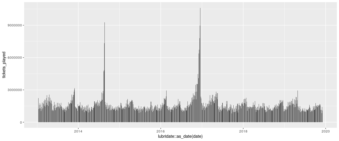
しかし、もっと面白いのは、ジャックポットに対するチケットの枚数をプロットすることが出来ることかもしれません。
# You can test your SQL here, but because we need to get the entire
# swisslos_jackpots table, we might just as well join it in R
three_correct_jp <- three_correct %>%
  left_join(dbGetQuery(griddb, "SELECT * FROM swisslos_jackpots;"), by = "date")

three_correct_jp %>%
  ggplot(aes(x = tickets_played, y = jackpot)) +
  geom_point()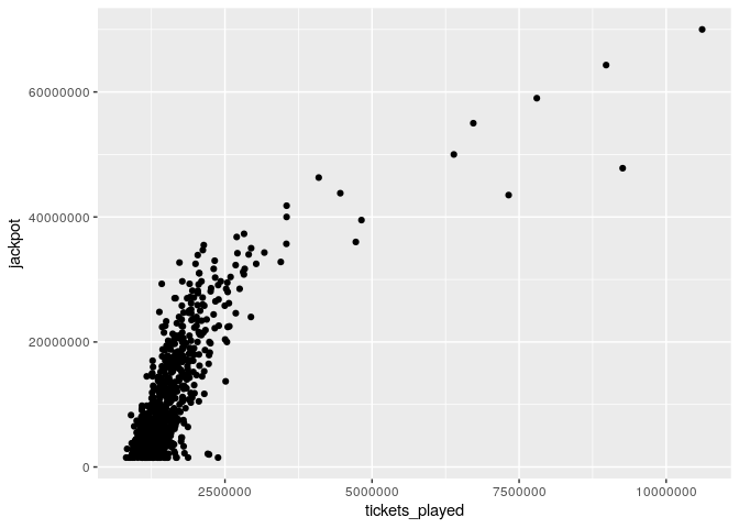
ジャックポットのサイズとプレイ枚数には、明らかに正の相関があることが分かります。
cor.test(three_correct_jp$tickets_played, three_correct_jp$jackpot)##
## Pearson's product-moment correlation
##
## data: three_correct_jp$tickets_played and three_correct_jp$jackpot
## t = 33.147, df = 718, p-value < 0.00000000000000022
## alternative hypothesis: true correlation is not equal to 0
## 95 percent confidence interval:
## 0.7470597 0.8050008
## sample estimates:
## cor
## 0.7776764
(この質問に簡単に答えるために、私たちは、人々が42分の6を完全にランダムにプレイしていると仮定しました。しかし、その効果は、プレイヤーの数を測定する能力を妨げない程度に小さいはずです。)
最も頻繁に再生されるラッキーナンバーはどれですか?
最も頻繁に再生されるものを探すには
ラッキーナンバー のない6つの組合せのうち、3つの組合せの当選回数を ラッキーナンバー が当たった組合せの回数と比較します。データセットから正しい ラッキーナンバー が得られるので、各 ラッキーナンバー について、たくさんの推定量が得られ、ボックスプロットで表示することが出来ます。
# Again, when writing straight SQL which is required for GridDB at the moment,
# we want to make it as easy as possible for ourselves.
# break SQL down into easy to understand snippets and combine
# I think it's a good idea to avoid nested str_interp and only use them
# for R computation
get_n_lucky <- function(conn, n) {
  # Add lucky and regular winners for n
  q_combined_counts <- paste(
    "SELECT SUM(winners) AS winners, date",
    "FROM swisslos_payouts",
    "WHERE combination = '${n}' OR combination = '${n} + 1'",
    "GROUP BY date"
  )

  # Only get lucky
  q_lucky_counts <- paste(
    "SELECT winners AS lucky, date",
    "FROM swisslos_payouts",
    "WHERE combination = '${n} + 1'"
  )

  # Combine lucky and regular counts
  q_lucky_and_regular_counts <- paste(
    "SELECT a.winners AS winners_count, b.lucky AS lucky_count, a.date AS date",
    "FROM (", q_combined_counts, ") a",
    "LEFT JOIN (", q_lucky_counts, ") b",
    "ON a.date = b.date",
    "ORDER BY a.date"
  )

  # Retrive lucky numbers
  q_lucky_numbers <- paste(
    "SELECT number AS lucky_number, date AS date",
    "FROM swisslos_numbers",
    "WHERE type = 'lucky'"
  )

  # Build the final query
  q_final <- paste(
    "SELECT winners_count, lucky_count, lucky_number, c.date AS date",
    "FROM (", q_lucky_and_regular_counts, ") c",
    "LEFT JOIN (", q_lucky_numbers, ") d",
    "ON c.date = d.date"
  )

  # Print the query if you want to know why building it up this way makes
  # a lot of sense

  dbGetQuery(conn, str_interp(q_final))
}

lucky_counts <- get_n_lucky(griddb, 3) %>%
  mutate(lucky_p = lucky_count / winners_count)

head(lucky_counts, n = 5)
## winners_count lucky_count lucky_number date lucky_p
## 1 60705 9174 4 2013-01-12 0.1511243
## 2 33745 5005 4 2013-01-16 0.1483183
## 3 43457 5810 6 2013-01-19 0.1336954
## 4 35013 6326 2 2013-01-23 0.1806757
## 5 48120 10718 3 2013-01-26 0.2227348
lucky_counts %>%
  ggplot(aes(x = factor(lucky_number), y = lucky_p, group = lucky_number)) +
  geom_boxplot() +
  geom_hline(yintercept = 1/6)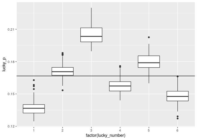
スイス人は ラッキーナンバー として 3 を好み、1 を嫌うのは明らかです。
最も頻繁に再生されるスタンダードナンバーはどれですか?
これは難しい問題です。ここでは、かなり直球でハチャメチャな方法を紹介しますので、より良い方法を考案してください。正解数4と正解数3の確率の間の係数が15.11であることを考えましょう。そこで、もし、データの中で、4つの正解数と3つの正解数の間の係数が大きければ、(平均して)引いた数字は弾かれる可能性が少し低く、係数が小さければ、弾かれた数字は弾かれる可能性が高いと考えられます。
# We can do all of this directly on our GridDB
# After we calculate the bias using the empirical frequencies and our
# swisslos_prob function, we combine the table with the numbers table and
# then we calculate the average bias for each number
get_3_and_4 <- function(conn) {
  # Three correct
  q_3 <- paste(
    "SELECT SUM(winners) AS w_3, date",
    "FROM swisslos_payouts",
    "WHERE combination = '3' OR combination = '3 + 1'",
    "GROUP BY date"
  )

  # Four correct
  q_4 <- paste(
    "SELECT SUM(winners) AS w_4, date",
    "FROM swisslos_payouts",
    "WHERE combination = '4' OR combination = '4 + 1'",
    "GROUP BY date"
  )

  # Combine the three counts and four counts tables
  q_w <- paste(
    "SELECT w_3, w_4, c.date AS date",
    "FROM (", q_3, ") c",
    "LEFT JOIN (", q_4, ") d",
    "ON c.date = d.date"
  )

  q_numbers <- paste(
    "SELECT number, date",
    "FROM swisslos_numbers",
    "WHERE type = 'normal'"
  )

  q_combine <- paste(
    "SELECT w_3 / w_4 - ${swisslos_prob(3) / swisslos_prob(4)} AS bias,",
    "number, a.date AS date",
    "FROM (", q_w, ") a",
    "LEFT JOIN (", q_numbers, ") b",
    "ON a.date = b.date"
  )

  q_final <- paste(
    "SELECT number, AVG(bias) AS bias",
    "FROM (", q_combine, ") e",
    "GROUP BY number"
  )

  dbGetQuery(conn, str_interp(q_final))
}

hacky <- get_3_and_4(griddb)
head(hacky)
## number bias
## 1 1 -0.4834515
## 2 2 -0.1532164
## 3 3 -0.4042146
## 4 4 -0.2777778
## 5 5 -0.3198068
## 6 6 -0.4269006
そこで、ちょっとハチャメチャなことをして、こんなことを思いつくのです。
# Centering and negating bias to make it look prettier
ggplot(hacky, aes(x = factor(number), y = -(bias - mean(bias)), fill = -bias)) + geom_col() +
  scale_fill_viridis_c() +
  theme(legend.position = "none")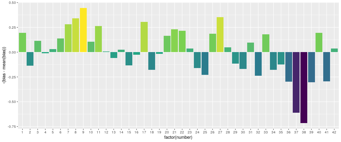
これがどれだけ正確かは分かりませんが、理にかなっています。1から12まで、1から31までの数字が誕生日になります。また、11、22、33も人気があることがわかります。では、どの数字をプレイすればいいのでしょうか?どれも、長い目で見れば損をすることになるからです。
dbDisconnect(griddb)## [1] TRUE