
概要
最近では、「インフレ」「品不足」「食品価格」「ガソリン価格」などの検索キーワードの人気が100~140%上昇しています(出典:Google Trends)。 世界中の人々が食料やガソリン価格の上昇を心配しているのは間違いありません。 食料、ガソリン、家庭用燃料などの物価の高騰が生活の質、特に少人数世帯に大きな影響を与えることは言うまでもありません。したがって、生存のための生活必需品の価格動向を分析し、情報を得ることが重要です。この重要な分析にGridDBとPythonを一緒に使ってみます。
jupyterのファイルへのリンクはこちらです。
https://github.com/griddbnet/Blogs/tree/inflation_cpi
データセットについて
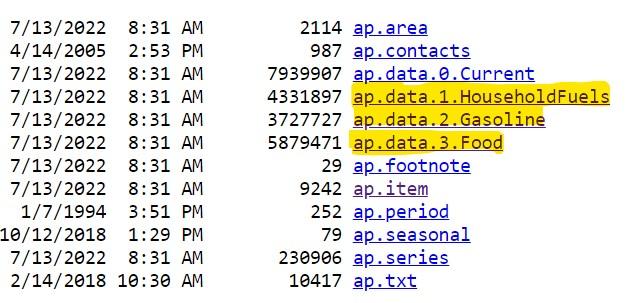
手元のデータセットは、U.S. Bureau Labor of Statisticsから取得した時系列データセットです。データセットはこちらからダウンロードできます。テキストファイルは、ウェブサイト内の「Average Price Data」セクションからダウンロードできます(下図参照)。

下の画像でハイライトされているテキストファイルが解析に使用されています 。
GridDBへのロード処理を計画する/データセットのサイズを把握する
データセットのサイズを把握することで、GridDBにデータをロードするプロセスを計画することができるのです。 これは、プログラムが動作しているシステム(クライアントシステム)に大きな負担をかけないために重要なことです。 このデータセットには40年以上のデータが含まれており、価格動向の分析を行うのに適しています。
import os
import numpy as np
import pandas as pd
import nums_from_string as ns
from IPython.core.display import Image, display
import seaborn as sns
from matplotlib import pyplot as plt
これらのテキストファイルは固定幅のファイルであることに注意してください。したがって、固定幅のファイルはpandasのread_fwf関数を使ってダウンロードする必要があります。
household_prices = pd.read_fwf('ap.data.1.HouseholdFuels.txt')
gasoline_prices = pd.read_fwf('ap.data.2.Gasoline.txt')
food_prices = pd.read_fwf('ap.data.3.Food.txt')
次に、データフレームが使用するメモリについて見てみましょう。
print('Size of household_prices', household_prices.info(memory_usage='deep'))
print('Size of food_prices', food_prices.info(memory_usage='deep'))
print('Size of gasoline_prices', gasoline_prices.info(memory_usage='deep'))
<class 'pandas.core.frame.DataFrame'>
RangeIndex: 103139 entries, 0 to 103138
Data columns (total 5 columns):
# Column Non-Null Count Dtype
--- ------ -------------- -----
0 series_id 103139 non-null object
1 year 103139 non-null int64
2 period 103139 non-null object
3 value 103139 non-null object
4 footnote_codes 0 non-null float64
dtypes: float64(1), int64(1), object(3)
memory usage: 20.4 MB
Size of household_prices None
<class 'pandas.core.frame.DataFrame'>
RangeIndex: 139986 entries, 0 to 139985
Data columns (total 5 columns):
# Column Non-Null Count Dtype
--- ------ -------------- -----
0 series_id 139986 non-null object
1 year 139986 non-null int64
2 period 139986 non-null object
3 value 139986 non-null object
4 footnote_codes 0 non-null float64
dtypes: float64(1), int64(1), object(3)
memory usage: 27.8 MB
Size of food_prices None
<class 'pandas.core.frame.DataFrame'>
RangeIndex: 88754 entries, 0 to 88753
Data columns (total 5 columns):
# Column Non-Null Count Dtype
--- ------ -------------- -----
0 series_id 88754 non-null object
1 year 88754 non-null int64
2 period 88754 non-null object
3 value 88754 non-null float64
4 footnote_codes 0 non-null float64
dtypes: float64(2), int64(1), object(2)
memory usage: 13.0 MB
Size of gasoline_prices None
上図のように、’house_prices’, ‘food_prices’, ‘gasoline_prices’ データセットをメモリにロードしたときのサイズはそれぞれ 22.7MB, 28.7MB, 18.5MB です。 この結果、合計69.9MBになりました。したがって、GridDBにデータをロードする際には、効率的なロード戦略が必要になります。
print(len(household_prices))
print(len(gasoline_prices))
print(len(food_prices))
103139
88754
139986
上記は、GridDBに処理/ロードされるレコード数の目安になります。
効率的なロード戦略としては、データを1000行ずつにチャンクし、一度に1チャンクずつGridDBにロードすることです。この場合、GridDB の API を複数回呼び出してデータをロードすることになります。 しかし、これによって読み込まれるデータをより細かく制御することができるようになります。また、データ全体を一度に読み込むこともできますが、その場合、多くのメモリと帯域幅を使用することになります(この場合、HTTP接続のタイムアウトが緩やかに設定されていることを確認してください)。
データクリーニング
GridDBにデータをロードする前に、データのクリーニングを行いましょう。
まず、データの種類を保存するための「Category」フィールドを追加しましょう。こうすることで、将来的に必要な場合に備えて、レコードの出所を特定することができます。
household_prices['Category'] = 'Household Commodities'
gasoline_prices['Category'] = 'Gasoline'
food_prices['Category'] = 'Food'
それでは、不要な列を削除し、期間フィールドから月番号を抽出し、値フィールドのデータクリーニングを行ってすべてのデータが数値であることを確認し、最後にデータフレーム内の列を並べる関数を定義してみましょう。 これができたら、読み込んだ3つのデータセット(dataframe)に対して、この関数を呼び出します。
def data_cleaning (df):
    df.drop('footnote_codes', axis=1, inplace=True) # Delete the column 'footnote_codes'
    df['month'] = df['period'].str[-2:] #extract the month
    # DataType conversions
    df["month"] = pd.to_numeric(df["month"]) #convert to number
    df["value"] = df["value"].replace(['-'],0) #Replace values that have a '-' to a 0
    df["value"] = pd.to_numeric(df["value"]) #convert to number
    cols = list(df.columns.values)
    df = df[['series_id', 'year', 'period', 'value', 'month', 'Category']] #order the columns in the dataframe
    return df
#Invoke the cleaning function on the 3 dataframes
household_prices = data_cleaning(household_prices)
gasoline_prices = data_cleaning(gasoline_prices)
food_prices = data_cleaning(food_prices)GridDBにおけるContainer構造の作成
GridDBでのコンテナ作成については、GridDB WebAPIを参照してください。
これから、GridDBにデータを格納するコンテナを作成する作業を進めます。
import requests  # to make http calls
import http
http.client.HTTPConnection.debuglevel = 1 #Tip - to enable detailed logging of http calls; this is not needed in case you don't detailed logging
#Construct an object to hold the request headers (ensure that you replace the XXX placeholder with the correct value that matches the credentials for your GridDB instance)
header_obj = {"Authorization":"XXX","Content-Type":"application/json; charset=UTF-8","User-Agent":"PostmanRuntime/7.29.0"}
#Construct the base URL based on your GRIDDB cluster you'd like to connect to (ensure that you replace the placeholders in the URL below with the correct values that correspond to your GridDB instance)
base_url = 'https://[host]:[port]/griddb/v2/[clustername]/dbs/[database_name]'#Construct an object to hold the request body (i.e., the container that needs to be created)
data_obj = {
"container_name": "Inflation_CPI_Analysis",
"container_type": "COLLECTION",
"rowkey": False,
"columns": [
{
"name": "series_id",
"type": "STRING"
},
{
"name": "year",
"type": "INTEGER"
},
{
"name": "period",
"type": "STRING"
},
{
"name": "value",
"type": "FLOAT"
},
{
"name": "month",
"type": "INTEGER"
},
{
"name": "category",
"type": "STRING"
}
]
}
#Set up the GridDB WebAPI URL
url = base_url + '/containers'
#Invoke the GridDB WebAPI with the headers and the request body
x = requests.post(url, json = data_obj, headers = header_obj)これで、すべてのデータを格納するコンテナがGridDBに作成されました。データセット内に同じ項目が複数回(月ごと、年ごと)存在するため、series_idフィールドが一意にならないので、rowkeyをFalseに設定していることに注意してください。
GridDBでコンテナにデータを追加する/行を登録する
ローディングの戦略:データチャンクを作成する
以下の関数は、データフレームをJSONオブジェクトに変換し、それを1000行ずつの複数のチャンクにしています。
#Setup the URL to be used to invoke the GridDB WebAPI to register rows in the container created previously
url = base_url + '/containers/Inflation_CPI_Analysis/rows'

def create_chunks_to_load_to_GRIDDB(df):
    list_of_dataframes = np.array_split(df, len(df)/1000) #Returns a list of dataframes; here,# the chunk size is 1000
    for i in list_of_dataframes:
        df_json = i.to_json(orient='values')
        request_body = df_json
        x = requests.put(url, data=request_body, headers=header_obj) #Invoke the GridDB WebAPI using the request constructed
        print(x.text)
データをチャンクしてGridDBにロードする関数を用いて、今ある3つのデータセットをロードします。
create_chunks_to_load_to_GRIDDB(household_prices)create_chunks_to_load_to_GRIDDB(food_prices)create_chunks_to_load_to_GRIDDB(household_prices)クイックバリデーション&TQL入門
さて、データの読み込みが完了したので、分析を進めることにします。今回の分析では、GridDBのTQLと呼ばれるクエリ言語を使用しています。TQLについてもっと知りたい方は、こちらのリソースをご覧ください。また、TQLを素早く把握するためのYoutubeビデオチュートリアルもあります。 こちらをクリックするとビデオチュートリアルを見ることができます。 GridDB WebAPI ブログ (「Fetching Data」セクションを参照)に従い、TQL文のリクエストの基本構造を学びます。
以下のTQLクエリは、GridDBに挿入されたレコード数が、データロードに使用した3つのデータフレームのレコードの合計と同じかどうかを簡単にチェックするものです。
#Setup the URL to be used to invoke the GridDB WebAPI to retrieve data from the container
url = base_url + '/tql'

#Construct the request body which has the TQL that is to be used to retrieve the data
#Use the count function to get the number of records in the container
request_body = '[{"name":"Inflation_CPI_Analysis", "stmt":"SELECT count(*) ", "columns":[]}]'

#Invoke the GridDB WebAPI
x = requests.post(url, data=request_body, headers=header_obj)print(x.text)[{"columns":[{"name":"aggregationResult","type":"DOUBLE"}],"results":[[331879.0]]}]
print(len(household_prices) + len(food_prices) + len(gasoline_prices))331879
マッピングテーブルをデータフレームとして読み込む
以下は、ダウンロードするマッピングファイルです。
すべてのファイルはタブ区切りファイルであることに注意してください。これらのマッピングファイルは、必要に応じてコードの説明を参照するために使用することができます。これらはPythonに残り、GridDBに読み込まれることはありません。
item_mapping = pd.read_csv('ap.item_mapping.txt',sep='\t')
period_mapping = pd.read_csv('ap.period_mapping.txt',sep='\t')
seasonal_mapping = pd.read_csv('ap.seasonal_mapping.txt',sep='\t')
area_mapping = pd.read_csv('ap.area_mapping.txt',sep='\t')
series_mapping = pd.read_csv('ap.series_mapping.txt',sep='\t')
時系列トレンド解析
シナリオ1:インフレは米価にどのような影響を与えたか?
シリーズID APU0000701311 (Rice, white, long grain, precooked); APU0000701312 (Rice, white, long grain, uncooked) のデータを収集するためのクエリを記述しているところです。それぞれ1ポンドの重さです。季節調整はしていません。
#Setup the URL to be used to invoke the GridDB WebAPI to retrieve data from the container
url = base_url + '/tql'

#Construct the request body which has the TQL that is to be used to retrieve the data
# Getting data for series_id APU0000701311 (Rice, white, long grain, precooked); APU0000701312 (Rice, white, long grain, uncooked)
request_body = '[{"name":"Inflation_CPI_Analysis", "stmt":"SELECT * WHERE series_id = \'APU0000701311\' OR series_id = \'APU0000701312\'", "columns":[]}]'

#Invoke the GridDB WebAPI
data_req1 = requests.post(url, data=request_body, headers=header_obj)
data_req1
GridDB WebAPI 呼び出しから受け取ったレスポンスを処理し、レスポンスに含まれるデータを用いてデータフレームを構築します。それができたら、各年の平均値を得るために、年フィールドでデータをグループ化します。これをプロットすると視覚的に傾向を確認することができます。
#Process the response received and construct a Pandas dataframe with the data from the response
myJson = data_req1.json()
Rice_trends = pd.DataFrame(myJson[0]["results"], columns=[myJson[0]["columns"][0]["name"], myJson[0]["columns"][1]["name"], myJson[0]["columns"][2]["name"], myJson[0]["columns"][3]["name"],myJson[0]["columns"][4]["name"],myJson[0]["columns"][5]["name"]])
#Group the data by year and get the mean for each year
Avg_value_rice = pd.DataFrame(Rice_trends.groupby(['year'])['value'].mean())#Construct a line plot with the data
plt.rcParams["figure.figsize"] = [12,12]
plt.rcParams["figure.autolayout"] = True
ax = sns.lineplot(x="year", y="value", data=Avg_value_rice)
ax.tick_params(rotation=45)
ax.set_title('Fig.1 Scenario 1 - Time Series Trends of Rice Prices', fontsize = 18)
plt.xlabel('Year', fontsize=14)
plt.ylabel('Average value ($ per pound)', fontsize=14)
plt.show()
シナリオ1に対する洞察:インフレの米への影響
Fig.1の傾向から、以下のような知見が得られました。
- 1980年に米価が急騰した後、0.4単位で下落しています。
- 1987年と2003年は、他の年に比べて値が下がっているようです。
- 1987年は、過去最低の値を記録しています。
- 2020年以降、米価は0.75台から0.9台へと急騰していることが分かります。
シナリオ2:インフレは鶏肉価格にどのような影響を与えたか?
鶏肉は、鶏肉と卵を含むすべての品目を含みます。series_id APU0200FF1101 (chicken breast with bone); APU0300FF1101 (chicken breast boneless); APU0300706111 (Chicken whole); APU0300706211 (Chicken breast); APU0300706212 (Chicken legs); APU0300708111 (Eggs) のデータを収集するクエリーを記述することです。なお、データ通り、これらの項目は非季節調整済みです。価格は1ポンド(453.6gm)あたりのものです。
#Setup the URL to be used to invoke the GridDB WebAPI to retrieve data from the container
url = base_url + '/tql'

#Construct the request body which has the TQL that is to be used to retrieve the data
# Getting data for series_id APU0200FF1101 (chicken breast with bone); APU0300FF1101 (chicken breast boneless); APU0300706111 (Chicken whole); APU0300706211 (Chicken breast); APU0300706212 (Chicken legs); APU0300708111 (Eggs)
request_body = '[{"name":"Inflation_CPI_Analysis", "stmt":"SELECT * WHERE series_id = \'APU0200FF1101\' OR series_id = \'APU0300FF1101\' OR series_id = \'APU0300706111\' OR series_id = \'APU0300706211\' OR series_id = \'APU0300706212\' OR series_id = \'APU0300708111\' ", "columns":[]}]'

#Invoke the GridDB WebAPI
data_req2 = requests.post(url, data=request_body, headers=header_obj)
data_req2
GridDB WebAPI 呼び出しから受け取ったレスポンスを処理し、レスポンスに含まれるデータを用いてデータフレームを構築します。
それができたら、各年の平均値を得るために、年フィールドでデータをグループ化します。これをプロットすると視覚的に傾向を確認することができます。
#Process the response received and construct a Pandas dataframe with the data from the response
myJson = data_req2.json()
Poultry_trends = pd.DataFrame(myJson[0]["results"], columns=[myJson[0]["columns"][0]["name"], myJson[0]["columns"][1]["name"], myJson[0]["columns"][2]["name"], myJson[0]["columns"][3]["name"],myJson[0]["columns"][4]["name"],myJson[0]["columns"][5]["name"]])
#Group the data on a yearly basis and get the mean value for each year
Avg_value_poultry = pd.DataFrame(Poultry_trends.groupby(['year'])['value'].mean())#Construct a line plot with the data
plt.rcParams["figure.figsize"] = [12,12]
plt.rcParams["figure.autolayout"] = True
ax = sns.lineplot(x="year", y="value", data=Avg_value_poultry)
ax.tick_params(rotation=45)
ax.set_title('Fig.2 Scenario 2 - Time Series Trends of Poultry Prices',fontsize=18)
plt.xlabel('Year', fontsize=14)
plt.ylabel('Average value ($ per pound)', fontsize=14)
plt.show()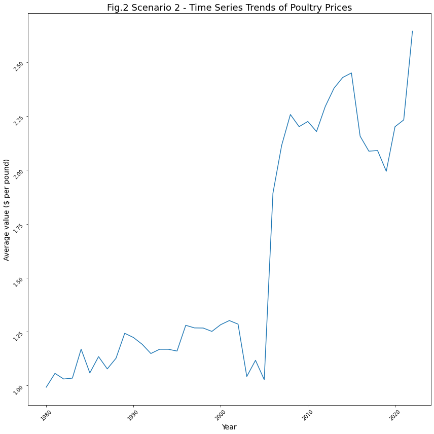
シナリオ2に対する洞察:インフレが家禽類に与える影響について
ここには、非常に興味深い傾向があります。Fig.2の傾向から、以下のような知見が得られました。
- 鶏肉の平均価格は、1980年から2005年までは1ポンドあたり1.0〜2.25円でした。しかし、2006年頃からは2.25に上昇しています。
- 2006年以降は、2.25以上に上昇しています。
シナリオ3:インフレは乳価にどのような影響を与えたか?
APU0000709111 – Milk, fresh, whole, fortified; APU0000709211 – Milk, fresh, skim; APU0000709212 – Milk, fresh, low fat; APU0200709111 – Milk, fresh, whole, fortified; APU0200709211 – Milk, fresh, skim .が考慮されます。なお、1.5ガロンで、季節調整されていない項目のみを考慮しました。
#Setup the URL to be used to invoke the GridDB WebAPI to retrieve data from the container
url = base_url + '/tql'

#Construct the request body which has the TQL that is to be used to retrieve the data
# Getting data for series_id APU0000709111 - Milk, fresh, whole, fortified; APU0000709211 - Milk, fresh, skim; APU0000709212 - Milk, fresh, low fat; APU0200709111 - Milk, fresh, whole, fortified; APU0200709211 - Milk, fresh, skim
request_body = '[{"name":"Inflation_CPI_Analysis", "stmt":"SELECT * WHERE series_id = \'APU0000709111\' OR series_id = \'APU0000709211\' OR series_id = \'APU0000709212\' OR series_id = \'APU0200709111\' OR series_id = \'APU0200709211\' ", "columns":[]}]'

#Invoke the GridDB WebAPI
data_req3 = requests.post(url, data=request_body, headers=header_obj)
data_req3
GridDB WebAPI 呼び出しから受け取ったレスポンスを処理し、レスポンスに含まれるデータを用いてデータフレームを構築します。 それができたら、各年の平均値を得るために、年フィールドでデータをグループ化します。これをプロットすると視覚的に傾向を確認することができます。
#Process the response received and construct a Pandas dataframe with the data from the response
myJson = data_req3.json()
Milk_trends = pd.DataFrame(myJson[0]["results"], columns=[myJson[0]["columns"][0]["name"], myJson[0]["columns"][1]["name"], myJson[0]["columns"][2]["name"], myJson[0]["columns"][3]["name"],myJson[0]["columns"][4]["name"],myJson[0]["columns"][5]["name"]])
#Group the data by rear and get the mean value for each year
Avg_value_milk = Milk_trends.groupby('year', as_index=False)['value'].mean()#Construct a line plot with the data; ensure that the ticks on the x axis are integer values
from matplotlib.ticker import MaxNLocator
plt.rcParams["figure.figsize"] = [12,12]
plt.rcParams["figure.autolayout"] = True
#year = (Milk_trends['year'])
ax = sns.lineplot(x="year", y="value", data=Avg_value_milk)
ax.tick_params(rotation=45)
ax.set_title('Fig.3 Scenario 3 - Time Series Trends of Milk Prices',fontsize=18)
ax.xaxis.set_major_locator(MaxNLocator(integer=True))
plt.xlabel('Year', fontsize=14)
plt.ylabel('Average value ($ per pound)', fontsize=14)
plt.show()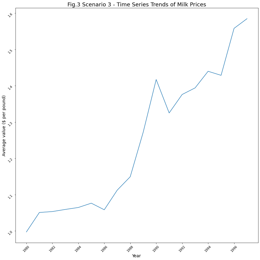
シナリオ3に対する洞察:インフレが牛乳に与える影響について
- 牛乳の平均価格は、1990年時点で1ポンドあたり約1.5ドルに上昇しました。
- 1980年から1986年の間、牛乳の平均価格は1ドルから1.1ドルの間でした。
- 1990年以降、平均価格は常に1.4ドル前後で推移しています。
シナリオ4:2022年のインフレ率はどうだったのか?
#Setup the URL to be used to invoke the GridDB WebAPI to retrieve data from the container
url = base_url + '/tql'

#Construct the request body which has the TQL that is to be used to retrieve the data
# Getting data for year 2022
request_body = '[{"name":"Inflation_CPI_Analysis", "stmt":"SELECT * WHERE year = 2022 ", "columns":[]}]'

#Invoke the GridDB WebAPI
data_req4 = requests.post(url, data=request_body, headers=header_obj)
data_req4
#Process the response received and construct a Pandas dataframe with the data from the response
myJson = data_req4.json()
year_2022_trends = pd.DataFrame(myJson[0]["results"], columns=[myJson[0]["columns"][0]["name"], myJson[0]["columns"][1]["name"], myJson[0]["columns"][2]["name"], myJson[0]["columns"][3]["name"],myJson[0]["columns"][4]["name"],myJson[0]["columns"][5]["name"]])#Construct a Seaborn lineplot with the data to display the trend lines for each category by month
import seaborn
sns.lineplot('month', 'value', ci=None, hue='category', data=year_2022_trends).set(title='Fig.4 Scenario 4 - How was 2022 in terms of inflation?')
plt.xlabel('Month (2022)', fontsize=14)
plt.ylabel('Average value ($ per unit)', fontsize=14)
plt.show()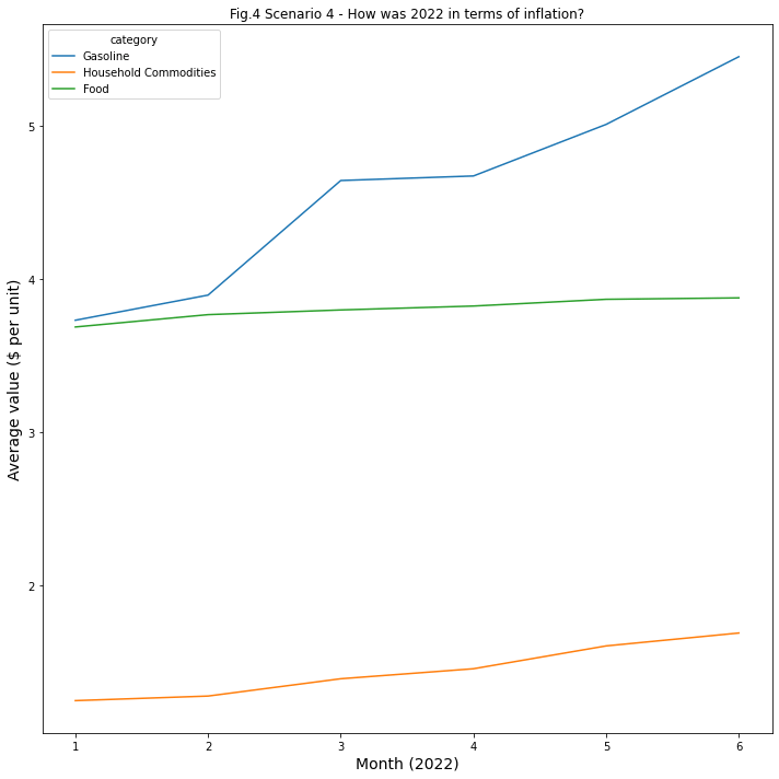
シナリオ4に対する洞察:2022年とインフレ率
2022年現在、1.ガソリンの価格はインフレの影響を受けているようです。2. 家庭用品や食料品の価格はインフレの影響をあまり受けていません。3.2022年2月よりガソリンが1個あたり0.5ドル値上げされました。4. 2022年3月現在ガソリンの価格は1個あたり1ドル値上がりしています。
シナリオ5:過去20年間、ガソリンの価格に季節性はあったのか?
#Setup the URL to be used to invoke the GridDB WebAPI to retrieve data from the container
url = base_url + '/tql'

#Construct the request body which has the TQL that is to be used to retrieve the data
# Getting data for the 'Gasoline' category for the last 20 years
request_body = '[{"name":"Inflation_CPI_Analysis", "stmt":"SELECT * WHERE year >= 2001 and year <= 2022 and category = \'Gasoline\'", "columns":[]}]'

#Invoke the GridDB WebAPI
data_req5 = requests.post(url, data=request_body, headers=header_obj)
data_req5
#Process the response received and construct a Pandas dataframe with the data from the response
myJson = data_req5.json()
gasoline_data_20_years = pd.DataFrame(myJson[0]["results"], columns=[myJson[0]["columns"][0]["name"], myJson[0]["columns"][1]["name"], myJson[0]["columns"][2]["name"], myJson[0]["columns"][3]["name"],myJson[0]["columns"][4]["name"],myJson[0]["columns"][5]["name"]])#Construct a boxplot of the year wise trends for the last 20 years
fig, ax = plt.subplots(nrows=1, ncols=1, figsize=(15, 6))
sns.boxplot(gasoline_data_20_years['year'], gasoline_data_20_years['value'], ax=ax)
ax.set_title('Fig.5 Scenario 5 - Year-wise trends', fontsize = 16, loc='center')
ax.set_xlabel('Year', fontsize = 12)
ax.set_ylabel('Value ($ per unit)', fontsize = 12)
plt.xticks(rotation=45)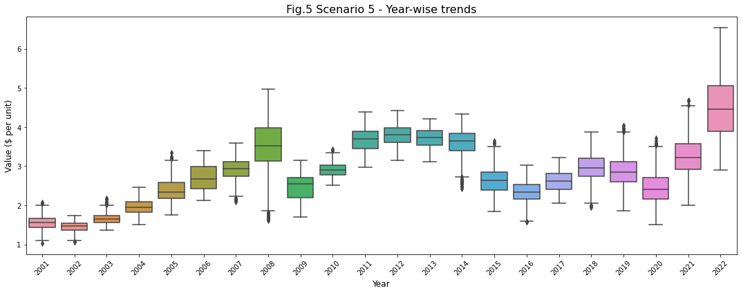
シナリオ5に対する洞察:過去20年間のインフレ率
- ガソリン価格のインフレ率に季節性は見られません。
- しかし、2022年には、インフレが過去最高水準になることは明らかです。
- プロットから分かるように、2008年は1年の大半を高値で推移していました。しかし、年末にかけて価格が急激に低下しています。このことは、2008年のボックスプロットの異常値からも明らかです。
- 2019年から2021年の間に、ガソリン価格の急激な上昇が何度かあったことが、上ひげを越える外れ値で観察されます。ガソリン価格の急激な上昇は、上ひげの外側にある異常値で観察されるように、何度もありました。
まとめ
上記のブログ記事では、GridDBを使って大量のデータを保存し、GridDBのTQLクエリ機能を使って効率的にデータを取得する方法を紹介しました。データの大きさにもかかわらず、データの読み込みはかなり高速(秒単位)でした。また、クエリ時間もかなり短く、数秒で結果を取得することができました。また、GridDBにコンテナを作成し、GridDBのコンテナに対してクエリを実行することが簡単にできることを実証できました。
ブログの内容について疑問や質問がある場合は Q&A サイトである Stack Overflow に質問を投稿しましょう。 GridDB 開発者やエンジニアから速やかな回答が得られるようにするためにも "griddb" タグをつけることをお忘れなく。 https://stackoverflow.com/questions/ask?tags=griddb