
データサイエンスの力は、技術やビジネスの課題解決にとどまりません。その使い道は、新しい技術を生み出すためのデータ分析、消費者に向けた広告、ビジネスにおける利益や売上の最大化などにとどまりません。オープンサイエンスのコンセプトにより、組織はデータを使って社会問題を処理するようになりました。人間の隠れた行動や文化的パターンに対して、統計的かつデータ主導の解決策を提供することが出来るのです。
我々は、サンフランシスコの犯罪部門のデータを使って、市民が報告する犯罪事件と、警察が報告する犯罪事件の関係を理解します。そして大量のデータを保存し、容易にアクセスできるようにするため、データベースプラットフォームとしてGridDBを使用します。
GridDBを使ったデータセットのエクスポートとインポート
GridDBは拡張性の高いインメモリデータベースであるため、並列処理により高いパフォーマンスと効率性を実現することが出来ます。GridDBのpythonクライアントを利用することで、GridDBとpythonを簡単に接続し、リアルタイムにデータのインポートやエクスポートに利用することが出来ます。
ライブラリ
いくつかのpythonライブラリを使用して、データの前処理と視覚的な分析を行います。
- Pandas: 特にデータフレームを扱う際に広く利用されているPythonライブラリ
- Matplotlib: 基本的なプロットを用いてデータを視覚的に表現するライブラリ
- Numpy: 数学的計算を伴うデータを扱うためのPythonライブラリ
前処理
犯罪データには 2 つのデータセットがあります。1 つは警察が報告した犯罪に関する情報を含むデータセットです。もう 1 つは警察署に寄せられた犯罪の通報に関する情報です。
incidents = pd.read_csv("datasets/downsample_police-department-incidents.csv")
calls = pd.read_csv("datasets/downsample_police-department-calls-for-service.csv")
データセットは、データフレームの形で変数 “incidents” と “calls” に保存されるようになりました。
データセットには分析上重要でないカラムがいくつか含まれているので、メモリ消費を最小限に抑え、分析の時間効率を最大にするために、データフレームからそれらを削除することにします。
incidents = incidents.drop(['IncidntNum', 'Time', 'X', 'Y', 'Location', 'PdId'], axis = 1)
calls = calls.drop(['Crime Id', 'Report Date', 'Offense Date', 'Call Time', 'Call Date Time',
                        'Disposition', 'Address', 'City', 'State', 'Agency Id','Address Type',
                        'Common Location'], axis = 1)
分析に使用するデータフレームに残っているカラムについて紹介します。
Incidents データフレーム:
- Category: 犯罪の種類
- Descript: 発生した犯罪事件の内容
- DayOfWeek: 犯行が行われた日
- Date: 犯罪が発生した日付
- PdDistrict: 犯罪が行われたサンフランシスコの地区
- Resolution: 犯罪に対してとった行動
- Address: 犯罪が行われた正確な場所
Calls データフレーム:
- Descript: 報告者が記述した犯罪の内容
- Date: 通報電話を受けた日。
また、それぞれの行を個別に追跡できるように、両方のデータフレームに主キーカラムを導入する必要があります。インデックスをリセットして、名前を ‘ID’ に変更します。
incidents.reset_index(drop=True, inplace=True)
incidents.index.name = 'ID'
incidents.dropna(inplace = True)

calls.reset_index(drop=True, inplace=True)
calls.index.name = 'ID'
calls.dropna(inplace = True)
クリーニングが完了したら、データフレームをCSVファイルとしてローカルドライブに保存し、GridDBにアップロードします。
#save it into csv
incidents.to_csv("preprocessed_incidents.csv")
calls.to_csv("preprocessed_calls.csv")
データセットをGridDBにエクスポートする
次に、GridDBにデータをアップロードします。そのために、前処理されたCSVファイルをpandasを使って読み込み、個別のdataframeに保存します。
#read the cleaned data from csv
incident_processed = pd.read_csv("preprocessed_incidents.csv")
calls_processed = pd.read_csv("preprocessed_calls.csv")
行情報を挿入する前に、2つのデータベースのデザインを生成できるように、GridDBにカラム情報を渡すための2つの異なるコンテナを作成します。
#Create container
incident_container = "incident_container"

# Create containerInfo
incident_containerInfo = griddb.ContainerInfo(incident_container,
                    [["ID", griddb.Type.INTEGER],
                    ["Category", griddb.Type.STRING],
                    ["Descript", griddb.Type.STRING],
                    ["DayOfWeek", griddb.Type.STRING],
                    ["Date", griddb.Type.TIMESTAMP],
                    ["PdDistrict", griddb.Type.STRING],
                    ["Resolution", griddb.Type.STRING]],
                    griddb.ContainerType.COLLECTION, True)

incident_columns = gridstore.put_container(incident_containerInfo)
#Create container
calls_container = "calls_container"
# Create containerInfo
calls_containerInfo = griddb.ContainerInfo(calls_container,
[["ID", griddb.Type.INTEGER],
["Descript", griddb.Type.STRING],
["Date", griddb.Type.TIMESTAMP]],
griddb.ContainerType.COLLECTION, True)
calls_columns = gridstore.put_container(calls_containerInfo)最後に、作成したスキーマに行を挿入します。
# Put rows
incident_columns.put_rows(incident_processed)

print("Data Inserted using the DataFrame")
# Put rows
calls_columns.put_rows(calls_processed)
print("Data Inserted using the DataFrame")GridDBからデータセットをインポートする
GridDBデータベースからデータを取得するために、SQLコマンドに似たTQLを使用します。データを取得する前に、データフレームに保存する前に、データの行を抽出するコンテナを作成することになります。
# Define the container names
    incident_container = "incident_container"

    # Get the containers
    obtained_data = gridstore.get_container(incident_container)

    # Fetch all rows - language_tag_container
    query = obtained_data.query("select *")

    rs = query.fetch(False)
    print(f"{incident_container} Data")
# Define the container names
call_container = "call_container"
# Get the containers
obtained_data = gridstore.get_container(call_container)
# Fetch all rows - language_tag_container
query = obtained_data.query("select *")
rs = query.fetch(False)
print(f"{call_container} Data")データ抽出の最後のステップは、カラム情報の順に行をクエリし、データの可視化と分析に使用するデータフレームに保存することです。
# Iterate and create a list
    retrieved_data= []
    while rs.has_next():
        data = rs.next()
        retrieved_data.append(data)

# Convert the list to a pandas data frame
    incidents = pd.DataFrame(retrieved_data,
                        columns=['ID', 'Category', 'Descript', 'DayOfWeek', 'Date',
                                 'PdDistrict', 'Resolution','Address'])
# Iterate and create a list
retrieved_data= []
while rs.has_next():
data = rs.next()
retrieved_data.append(data)
# Convert the list to a pandas data frame
calls = pd.DataFrame(retrieved_data,
columns=['ID', 'Descript', 'Date'])“incidents” と “calls” の 2 つのデータフレームとして保存され、データ分析のためにクリーンアップされたデータが利用可能になりました。
データ解析と可視化
まず、グループ化されたデータを数えるのに役立つNullまたはゼロ値で構成される列を導入して分析を始めます。
incidents['NumOfIncidents'] = np.zeros(len(incidents))
calls['NumOfCalls'] = np.zeros(len(calls))
報告された犯罪は、警察自身によって報告されながら、異なるカテゴリーに属しています。では、そのデータをもとに、サンフランシスコで起こる主な犯罪を見ていきましょう。
incident_categories = incidents.groupby(["Category"]).count()
n_largest = incident_categories['NumOfIncidents'].nlargest(n=10)
incident_categories.reset_index(inplace = True)
incident_categories = incident_categories[["Category","NumOfIncidents"]]
n_largest.plot(kind = 'barh')
plt.show()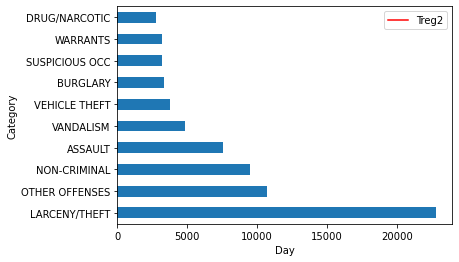
サンフランシスコで起こる犯罪のほとんどは、「窃盗」に関連していることがわかります。この調査をさらに進めて、この犯罪が多く発生している地域を調べることも出来ます。
Theft_address = incidents[incidents['Category']=="LARCENY/THEFT"]
Theft_address = Theft_address.groupby(["Address"]).count()
n_largest = Theft_address['NumOfIncidents'].nlargest(n=10)
Theft_address.reset_index(inplace = True)
Theft_address = Theft_address[["Address","NumOfIncidents"]]
n_largest.plot(kind = 'barh')
plt.show()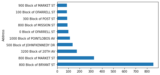
ここで、毎日の事件と毎日の通話の値が時間とともにどのように変化しているかを知るために、警察から報告された毎日の通話と毎日の事件を個別に調査してみます。キーからDate列を削除することで、結果は、両方のケースで各日付の観察に対して複数の行を持つ細長いデータフレームになります。
daily_incidents = incidents.groupby(["Date"]).count()
daily_incidents.reset_index(inplace = True)
daily_incidents = daily_incidents[["Date","NumOfIncidents"]]


daily_calls = calls.groupby(["Date"]).count()
daily_calls.reset_index(inplace = True)
daily_calls = daily_calls[["Date","NumOfCalls"]]
次に、特定の日付における通話とインシデントの値を1つのデータフレームで取得するために、日付カラムで両方のデータフレームを結合します。
shared_dates = pd.merge(daily_incidents, daily_calls, on='Date', how = 'inner')両列を散布図にプロットし、線形回帰モデルを適用して、データが示すパターンの直線を得ましょう。そのために、まずデータを回帰モデルに適合させ、そのデータ点を使って散布図を描き、次にモデルによって得られたデータ点を使って直線を描き、”Treg1″ として保存することにします。
d1 = np.polyfit(shared_dates.index,shared_dates['NumOfCalls'],1)
f1 = np.poly1d(d1)
shared_dates.insert(3,'Treg1',f1(shared_dates.index))
ax = shared_dates.plot.scatter(x = 'Day', y='NumOfCalls')
shared_dates.plot(y='Treg1',color='Red',ax=ax)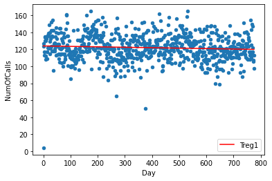
同様に、2つ目の列についても別の線形モデルを作成し、モデルのデータポイントを “Treg2” カラムに保存します。
d2 = np.polyfit(shared_dates.index,shared_dates['NumOfIncidents'],1)
f2 = np.poly1d(d2)
shared_dates.insert(4,'Treg2',f2(shared_dates.index))
ax = shared_dates.plot.scatter(x='Day' ,y='NumOfIncidents')
shared_dates.plot(y='Treg2',color='Red',ax=ax)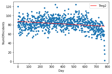
2 つの変数の関係をさらに調査し、定量化するために、相関係数のテクニックを使用します。統計学で最もシンプルで使用されているピアソン相関係数を使用します。これは-1から+1まで変化し、-1は強い負の相関、+1は強い正の相関を示します。Pythonの’corr’関数のデフォルト変数として使用されます。
correlation = shared_dates['NumOfIncidents'].corr(shared_dates['NumOfCalls'])相関係数は0.1469688であり、2つの変数の間には非常に弱い正の相関があることが分かります。
結論
統計的には、警察が通報する事件の数は、警察が受けた通報の数に左右されないと結論付けられます。また、サンフランシスコの中でも特に治安の悪い地域を抽出し、警察による特別な警備が必要であることが分かりました。すべての分析は、バックエンドでGridDBデータベースを使用して行われたため、シームレスかつ効率的に統合することができました。
ブログの内容について疑問や質問がある場合は Q&A サイトである Stack Overflow に質問を投稿しましょう。 GridDB 開発者やエンジニアから速やかな回答が得られるようにするためにも "griddb" タグをつけることをお忘れなく。 https://stackoverflow.com/questions/ask?tags=griddb