
概要
米国には、大手風力発電機メーカーやエンジニアリングチームが設計・施工した最新鋭の風力発電機がいくつも点在しています。 eia.gov によると、米国における全発電量の約9.2%が風力発電によるものであることが分かりました。興味深いデータセットを手に、堅牢なデータベースと組み合わせて、米国の風力タービンを分析することにします。
データセットについて
米国風力タービンデータベース(USWTDB)は、米国内の陸上および洋上の風力タービンの位置、対応する風力プロジェクト情報、タービンの技術仕様などを提供するデータセットです。このデータベースは、米国エネルギー省(DOE)の風力エネルギー技術局(WETO)、ローレンス・バークレー国立研究所(LBNL)の電力市場・政策グループ、米国地質調査所(USGS)のエネルギー資源プログラム、米国クリーンパワー協会(ACP)が共同出資して作成したものです。
全米44州(+グアム、PR)に72,130基のタービンが設置されています。
データは https://eerscmap.usgs.gov/uswtdb/data/からダウンロードできます。
データの収集方法については、https://eta-publications.lbl.gov/sites/default/files/uswtdb_v5_1_20220729_memo.pdfを参照してください。
データセットの引用元について
Hoen, B.D., Diffendorfer, J.E., Rand, J.T., Kramer, L.A., Garrity, C.P., and Hunt, H.E., 2018, United States Wind Turbine Database v5.1 (July 29, 2022): U.S. Geological Survey, American Clean Power Association, and Lawrence Berkeley National Laboratory data release, https://doi.org/10.5066/F7TX3DN0.
データセット変数に関するメモ
◘ case_id:一意のuswtdb ID
◘ faa_ors – デジタル障害物ファイルID
◘ faa_asn – 航空学研究番号
◘ usgs_pr_id – USGS ID
◘ t_state – タービンが設置されている州
◘ eia_id – プラントID
◘ t_county – タービンが設置されている郡
◘ t_fips – タービンが設置されている州および郡
◘ p_name:タービンの名称
◘ p_year:プロジェクトが稼働した年
◘ p_tnum-プロジェクトに含まれるタービンの数
◘ p_cap-プロジェクトの容量(メガワット)
◘ t_manu – タービンOEM
◘ t_model – タービンモデル
◘ t_cap – タービン容量(キロワット)
◘ t_hh – タービンハブ高(メートル)
◘ t_rd – タービンローター直径(メートル)
◘ t_rsa – タービンローター掃気面積(平方メートル)
◘ t_ttlh – タービン全高(メートル)
◘ retrofit – タービンの建設当初からの改修の有無。(0-レトロフィットなし、1-レトロフィットあり)
◘ retrofit_year – タービンがレトロフィットされた場合、レトロフィットの年
◘ t_conf_atr – 提供された属性に対する信頼度を示す順序変数
◘ t_conf_loc – 位置情報信頼性
◘ t_img_date – タービン位置の目視確認に使用した画像の日付(NAIPが画像ソースの場合、月と日は01/01に設定されていることに注意)
◘ t_img_srce – タービン位置を目視確認するための画像ソース
◘ xlong – 経度(10進法)
◘ ylat – 緯度(10進法)
コードブックのダウンロードは こちらからどうぞ。
全体的な前提
このブログ記事の大前提は、GridDBの以下の興味深い機能を利用することです。
- GridDBのTQL機能による集計データの取得。
- GridDBのSQL機能として、サブクエリ、事例文、節別グループ、節ありを用いたデータ取得やネストされたサブクエリを使用して、複数のデータポイントをよく取得します。
GridDBには、「Collections」コンテナと「Time Series」コンテナという2種類のコンテナがあります。GridDBが提供する様々なタイプのコンテナについて詳しく知りたい方は、こちらの記事を参照してください。 「GridDBを使用したデータモデリング」
GridDBは、コンテナからデータを取得する仕組みも複数用意しています。SQLだけでなくTQLもサポートしており、データを取得することができます。ここでは、様々なシナリオを想定し、GridDBコンテナからそのシナリオに沿ったデータを取得する方法を紹介します。
まずは、GridDB クラウドサブスクリプションを取得することを忘れないでください。
必要な基本ライブラリのロード
import os
import numpy as np
import pandas as pd
import nums_from_string as ns
from IPython.core.display import Image, display
import seaborn as sns
from matplotlib import pyplot as plt
from mapboxgl.utils import *
from mapboxgl.viz import *
from matplotlib.dates import DateFormatter
import plotly.graph_objects as go # For the map
sns.set()
C:\Users\mg_su\anaconda3\lib\site-packages\scipy\__init__.py:146: UserWarning: A NumPy version >=1.16.5 and <1.23.0 is required for this version of SciPy (detected version 1.23.1
warnings.warn(f"A NumPy version >={np_minversion} and <{np_maxversion}"
注意点
- コンテナ内の列の順序は、データフレーム内の列の順序と同じであるべきであることを覚えておくことが重要です。これは、任意のリレーショナルデータベースにおけるInsert操作に似ています。
Turbine_Data = pd.read_excel("Turbine_Data.xlsx", header=0,keep_default_na=True, index_col=None)# Dropping rows that have the operational year (p_year) that are empty
print(len(Turbine_Data))
Turbine_Data.dropna(subset=['p_year'],inplace=True)
print(len(Turbine_Data))72130
71398
欠測値のインプットとデータ型変換
#Check for missing values and fill it
Turbine_Data.fillna(Turbine_Data.median(),inplace=True)
Turbine_Data.head()
C:\Users\mg_su\AppData\Local\Temp/ipykernel_13828/1904398437.py:2: FutureWarning: DataFrame.mean and DataFrame.median with numeric_only=None will include datetime64 and datetime64tz columns in a future version.
Turbine_Data.fillna(Turbine_Data.median(),inplace=True)
C:\Users\mg_su\AppData\Local\Temp/ipykernel_13828/1904398437.py:2: FutureWarning: Dropping of nuisance columns in DataFrame reductions (with 'numeric_only=None') is deprecated; in a future version this will raise TypeError. Select only valid columns before calling the reduction.
Turbine_Data.fillna(Turbine_Data.median(),inplace=True)
#Convert the datatypes of the data as needed
Turbine_Data['t_img_date'] = Turbine_Data['t_img_date'].astype(str)
Turbine_Data['usgs_pr_id'] = Turbine_Data['usgs_pr_id'].astype(str)
Turbine_Data['eia_id'] = Turbine_Data['eia_id'].astype(str)
Turbine_Data['t_cap'] = Turbine_Data['t_cap'].astype(str)
Turbine_Data.dtypes
case_id int64
faa_ors object
faa_asn object
usgs_pr_id object
eia_id object
t_state object
t_county object
t_fips int64
p_name object
p_year float64
p_tnum int64
p_cap float64
t_manu object
t_model object
t_cap object
t_hh float64
t_rd float64
t_rsa float64
t_ttlh float64
retrofit int64
retrofit_year float64
t_conf_atr int64
t_conf_loc int64
t_img_date object
t_img_srce object
xlong float64
ylat float64
dtype: object
#Manipulate the data as needed
Turbine_Data['p_year'] = Turbine_Data['p_year'].astype(int).astype(str) # Convert from an integer to a string
Turbine_Data['p_year'] = Turbine_Data['p_year'] + '-01-01T00:00:00.000Z' # Append '-01-01' to it
col = Turbine_Data.pop("p_year") # Pop the column and store it in the variable 'col'
Turbine_Data.insert(0, col.name, col) #Re-insert the column as the first column of the dataframe
Turbine_Data.head()# Extracting column headers for the GridDB WebApi Container structure
col_vals = (list(Turbine_Data.columns.values))
col_dtypes = (list(Turbine_Data.dtypes))
data_tuples = list(zip(col_vals,col_dtypes)) # Binding lists to a tuple
# Converting list of tuples to pandas dataframe
container_columns = pd.DataFrame(data_tuples, columns=['col_vals','col_datatypes'])
container_columns.to_csv('container_columns.csv',index=False)
container_columns #column names for the containerファイル ‘container_columns’ には、すべてのヘッダとそのデータ型が含まれています。 最後に、Python のデータ型から GridDB のデータ型に変更します。 GridDBがサポートするデータ型とそれぞれの表記については、こちらをご覧ください。
GridDBにデータを格納するコンテナを設定する
GridDBでのコンテナ作成については、GridDBのこちらの リソースを参照してください。
import requests  # to make http calls
import http
http.client.HTTPConnection.debuglevel = 1 #Tip - to enable detailed logging of http calls; this is not needed in case you don't detailed logging
なお、base_urlを作成する際に、コンテナ名は必要ありません。
#Construct an object to hold the request headers (ensure that you replace the XXX placeholder with the correct value that matches the credentials for your GridDB instance)
header_obj = {"Authorization":"XXX","Content-Type":"application/json; charset=UTF-8","User-Agent":"PostmanRuntime/7.29.0"}

#Construct the base URL based on your GridDB cluster you'd like to connect to (ensure that you replace the placeholders in the URL below with the correct values that correspond to your GridDB instance)
#'https://[host]:[port]/griddb/v2/[clustername]/dbs/[database_name]'
base_url = 'https://[host]/griddb/v2/[clustername]/dbs/[databasename]'
#Construct an object to hold the request body (i.e., the container that needs to be created)
data_obj = {
"container_name": "Wind_Turbine_Data",
"container_type": "COLLECTION",
"rowkey": False,
"columns": [
{
"name": "p_year",
"type": "TIMESTAMP"
},
{
"name": "case_id",
"type": "INTEGER"
},
{
"name": "faa_ors",
"type": "STRING"
},
{
"name": "faa_asn",
"type": "STRING"
},
{
"name": "usgs_pr_id",
"type": "STRING"
},
{
"name": "eia_id",
"type": "STRING"
},
{
"name": "t_state",
"type": "STRING"
},
{
"name": "t_county",
"type": "STRING"
},
{
"name": "t_fips",
"type": "INTEGER"
},
{
"name": "p_name",
"type": "STRING"
},
{
"name": "p_tnum",
"type": "INTEGER"
},
{
"name": "p_cap",
"type": "FLOAT"
},
{
"name": "t_manu",
"type": "STRING"
},
{
"name": "t_model",
"type": "STRING"
},
{
"name": "t_cap",
"type": "STRING"
},
{
"name": "t_hh",
"type": "STRING"
},
{
"name": "t_rd",
"type": "STRING"
},
{
"name": "t_rsa",
"type": "STRING"
},
{
"name": "t_ttlh",
"type": "STRING"
},
{
"name": "retrofit",
"type": "INTEGER"
},
{
"name": "retrofit_year",
"type": "STRING"
},
{
"name": "t_conf_atr",
"type": "INTEGER"
},
{
"name": "t_conf_loc",
"type": "INTEGER"
},
{
"name": "t_img_date",
"type": "STRING"
},
{
"name": "t_img_srce",
"type": "STRING"
},
{
"name": "xlong",
"type": "FLOAT"
},
{
"name": "ylat",
"type": "FLOAT"
}
]
}
#Set up the GridDB WebAPI URL
url = base_url + '/containers'
#Invoke the GridDB WebAPI with the headers and the request body
x = requests.post(url, json = data_obj, headers = header_obj)GridDBコンテナへのデータロード(行の登録)
Pandasの ‘to_json’ 関数は、コンテナへのデータロードに使用されるリクエストボディを構築するために使用されます。 コンテナに行を追加するために必要なフォーマットの詳細については、こちらの記事を参照してください。
#Convert the data in the dataframe to the JSON format
Turbine_Data_json = Turbine_Data.to_json(orient='values')
request_body = Turbine_Data_json
url は、ベース url と新しく作成されたコンテナ名で構成されます。(この場合、’Wind_Turbine_Data’)
#Setup the URL to be used to invoke the GridDB WebAPI to register rows in the container created previously
url = 'https://[server]/griddb/v2/[clusterName]/dbs/[databasename]/containers/Wind_Turbine_Data/rows'

#Invoke the GridDB WebAPI using the request constructed
x = requests.put(url, data=request_body, headers=header_obj)
2000年以降に稼働したタービンは何基ですか?
#Construct the SQL to be used
sql = ("SELECT p_year, count(*) as cnt FROM Wind_Turbine_Data where p_year >=TIMESTAMP('2000-01-01T00:00:00.000Z') group by p_year")
#Setup the URL to be used to invoke the GridDB WebAPI to retrieve data from the container
url = base_url + '/sql'#Construct the request body
request_body = '[{"type":"sql-select", "stmt":"'+sql+'"}]'#Validate the constructed request body
request_body'[{"type":"sql-select", "stmt":"SELECT p_year, count(*) as cnt FROM Wind_Turbine_Data where p_year >=TIMESTAMP(\'2000-01-01T00:00:00.000Z\') group by p_year"}]'
GridDB SQL API を呼び出して結果を取得し処理します。
#Invoke the GridDB WebAPI
data_req1 = requests.post(url, data=request_body, headers=header_obj)#Process the response received and construct a Pandas dataframe with the data from the response
myJson = data_req1.json()
Turbines_after_2000 = pd.DataFrame(myJson[0]["results"], columns=[myJson[0]["columns"][0]["name"], myJson[0]["columns"][1]["name"]])
Turbines_after_2000=Turbines_after_2000.sort_values(by=['cnt'], ascending=False)#Plot the data as a bar plot
Turbines_after_2000['year_formatted'] = pd.to_datetime(Turbines_after_2000['p_year'])
Turbines_after_2000['year'] = pd.DatetimeIndex(Turbines_after_2000['year_formatted']).year
fig,ax = plt.subplots(figsize=(9,6))
sns.barplot(Turbines_after_2000['year'], Turbines_after_2000['cnt'], ax=ax,order=Turbines_after_2000.sort_values('cnt',ascending = False).year)
ax.set_title('Number of Turbines by Year', fontsize = 16, loc='center')
ax.set_xlabel('Year', fontsize = 12)
ax.set_ylabel('Number of Turbines', fontsize = 12)
plt.xticks(rotation=45)
plt.show()C:\Users\mg_su\anaconda3\lib\site-packages\seaborn\_decorators.py:36: FutureWarning: Pass the following variables as keyword args: x, y. From version 0.12, the only valid positional argument will be `data`, and passing other arguments without an explicit keyword will result in an error or misinterpretation.
warnings.warn(
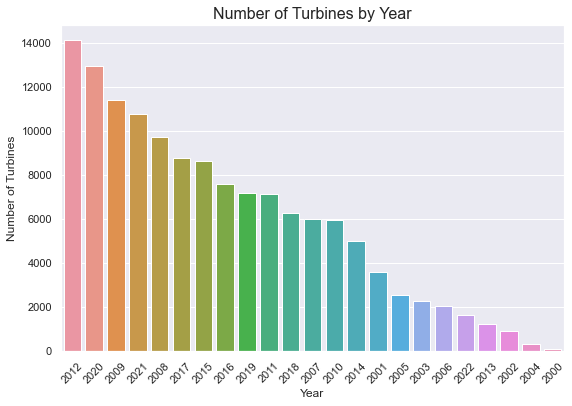
インサイト
◘ 2012 年は、7000 基以上のタービンが稼動し、最も多くのタービンが稼動した年であった。
◘ 2020 年頃には、6000 基以上のタービンが稼動する。
◘ 2000 年は、稼働したタービン・プロジェクトが最も少なかった年である。
各プロジェクトの平均的なタービンの数は?
このデータを取得するために、GridDB の tql 機能を使用して集計を実行し、平均的なタービン数を取得します。
GridDB TQL API を呼び出して、結果の取得と処理を行います。
#Setup the URL to be used to invoke the GridDB WebAPI to retrieve data from the container
url = base_url + '/tql'
#Construct the request body which has the TQL that is to be used to retrieve the data
# Getting data for series_id APU0000709111 - Milk, fresh, whole, fortified; APU0000709211 - Milk, fresh, skim; APU0000709212 - Milk, fresh, low fat; APU0200709111 - Milk, fresh, whole, fortified; APU0200709211 - Milk, fresh, skim
request_body = '[{"name":"Wind_Turbine_Data", "stmt":"SELECT AVG(p_tnum) ", "columns":[]}]'
#Invoke the GridDB WebAPI
data_req2 = requests.post(url, data=request_body, headers=header_obj)
data_req2#Process the response received and construct a Pandas dataframe with the data from the response
myJson = data_req2.json()
Avg_Num_Turbines = pd.DataFrame(myJson[0]["results"], columns=[myJson[0]["columns"][0]["name"]])print('The average number of turbines created per project is', Avg_Num_Turbines['aggregationResult'][0])The average number of turbines created per project is 105.33435984616243
200基以上のタービンを建設しているタービンメーカーは?
GridDBのエイリアス名は、一部のリレーショナルデータベースとは異なり、引用符で囲む必要がないことに注意してください。
タービンの数を集計する SQL クエリを作成します。このクエリは、メーカーに基づいてデータをグループ化し、200 台以上のタービンを持つメーカーに結果を限定するために having 節を持ちます。
#Construct the SQL to be used
sql = ("SELECT t_manu,SUM(p_tnum) as Total_Turbines FROM Wind_Turbine_Data where t_manu is NOT NULL GROUP BY t_manu HAVING SUM(p_tnum) >=200")GridDB API を起動し、結果を取得・処理します。
#Setup the URL to be used to invoke the GridDB WebAPI to retrieve data from the container
url = base_url + '/sql'
#Construct the request body which has the SQL that is to be used to retrieve the data
request_body = '[{"type":"sql-select", "stmt":"'+sql+'"}]'
#Invoke the GridDB WebAPI
data_req4 = requests.post(url, data=request_body, headers=header_obj)
data_req4#Process the response received and construct a Pandas dataframe with the data from the response
myJson = data_req4.json()
manufacturers_and_models = pd.DataFrame(myJson[0]["results"], columns=[myJson[0]["columns"][0]["name"],myJson[0]["columns"][1]["name"]])その結果を表形式で表示してみましょう。
from tabulate import tabulate
print(tabulate(manufacturers_and_models, headers='keys', tablefmt='psql'))
+----+---------------------------------+------------------+
| | t_manu | Total_Turbines |
|----+---------------------------------+------------------|
| 0 | Enron | 105018 |
| 1 | Fuhrlander | 232 |
| 2 | DWT | 294 |
| 3 | NEG Micon | 42574 |
| 4 | Sany | 326 |
| 5 | Suzlon | 114410 |
| 6 | Acciona | 112956 |
| 7 | Alstom | 576 |
| 8 | China Creative Wind Energy | 578 |
| 9 | Micon | 89688 |
| 10 | Nordex | 225556 |
| 11 | Nordtank | 52680 |
| 12 | Bonus | 90196 |
| 13 | NedWind | 338 |
| 14 | Entegrity | 548 |
| 15 | Zond | 6526 |
| 16 | Vestas | 3704146 |
| 17 | Mitsubishi | 638562 |
| 18 | Siemens | 827166 |
| 19 | Goldwind Americas | 4608 |
| 20 | REpower | 72126 |
| 21 | GE Wind | 5963708 |
| 22 | Northern Power Systems | 457 |
| 23 | Siemens Gamesa Renewable Energy | 377154 |
| 24 | Goldwind | 18706 |
| 25 | DeWind | 4312 |
| 26 | Gamesa | 503372 |
| 27 | Clipper | 39508 |
+----+---------------------------------+------------------+
風力発電機の地理的な分布はどうなっているのでしょうか?
ヒント: GridDB では、エイリアス名を指定する際に ‘as’ キーワードは必要ありません。同様に、いくつかのリレーショナルデータベース・プラットフォームと同様に、サブクエリのためのエイリアス名を必要とします。
サブクエリを使用する SQL クエリを作成し、SQL case 文を使用して、データを異なるビンまたはグループに分類します。このビンは、後ほど可視化する際に使用します。
#Construct the sub-query SQL to be used
sql = ("SELECT t_manu,p_name,Turbine_Num, xlong,ylat, CASE WHEN Turbine_Num = 1 THEN '1 turbine' WHEN Turbine_Num >= 2 AND Turbine_Num <= 25 THEN '2-25 turbines' WHEN Turbine_Num >= 26 AND Turbine_Num <= 100 THEN '26-100 turbines' WHEN Turbine_Num >= 101 AND Turbine_Num <= 500 THEN '101-500 turbines' WHEN Turbine_Num >= 501 AND Turbine_Num <= 750 THEN '501-750 turbines' END Turbine_bins FROM (SELECT DISTINCT t_manu,p_name,xlong,ylat, Sum(p_tnum) Turbine_Num FROM Wind_Turbine_Data where t_manu is NOT NULL GROUP BY t_manu,p_name,xlong,ylat) t")
これからGridDBコンテナに対してSQLを実行し、その結果を取得して処理します。
#Setup the URL to be used to invoke the GridDB WebAPI to retrieve data from the container
url = base_url + '/sql'

#Construct the request body which has the SQL that is to be used to retrieve the data
request_body = '[{"type":"sql-select", "stmt":"'+sql+'"}]'

#Invoke the GridDB WebAPI
data_req5 = requests.post(url, data=request_body, headers=header_obj)
#Process the response received and construct a Pandas dataframe with the data from the response
myJson = data_req5.json()
Turbine_Locations = pd.DataFrame(myJson[0]["results"], columns=[myJson[0]["columns"][0]["name"],myJson[0]["columns"][1]["name"],myJson[0]["columns"][2]["name"],myJson[0]["columns"][3]["name"],myJson[0]["columns"][4]["name"],myJson[0]["columns"][5]["name"]])
#Let's take a look at some of the data
Turbine_Locations.tail()#Create a list which will have the bin names
cut_labels = ['1 turbine','2-25 turbines', '26-100 turbines', '101-500 turbines', '501-750 turbines']データは取得され、ビンに分類され、データフレームで提供されています。 各ビンまたは分類について、データフレームをフィルタリングしてビンに対応するレコードを取得し、同じものを米国の地図上にプロットします。各ビンには異なる色が使用されます。
#Plot the data
scale = 55

fig = go.Figure()
limits = [(0,1),(2,25),(26,100),(101,500),(501,750)]
colors = ["maroon","cyan","lime","mediumorchid","royalblue"]

#plot the data for each bin
for i in range(len(limits)):

    lim = limits[i]

    #filter the dataframe to get the records for the current bin
    Turbine_Data_filtered = Turbine_Locations.loc[(Turbine_Locations['Turbine_bins'] == cut_labels[i])]

    #plot the data
    fig.add_trace(go.Scattergeo(
        locationmode = 'USA-states',
        lon = Turbine_Data_filtered['xlong'],
        lat = Turbine_Data_filtered['ylat'],
        text = Turbine_Data_filtered['p_name'],
        marker = dict(
            size = Turbine_Data_filtered['Turbine_Num']/scale,  #size of the marker will depend on the number of turbines
            color = colors[i],
            line_color='rgb(40,40,40)',
            line_width=0.5,
            sizemode = 'area'
        ),
        name = '{0} - {1}'.format(lim[0],lim[1])
        )
    )


fig.update_layout(
        title_text = 'Turbine Distribution in the United States',
        showlegend = True,
        geo = dict(
            scope = 'usa',
            landcolor = 'rgb(217, 217, 217)',
        )

    )

fig.update_layout(
    title={
        'y':0.9,
        'x':0.5,
        'xanchor': 'center',
        'yanchor': 'top'})

fig.show()
注意: 地図はインタラクティブで、各ドットにカーソルを合わせるとツールチップが表示され、詳細を確認することができます。投げ縄やズーム機能を使って、より詳しく知ることができます。
インサイト
◘ 国内には26基から500基のタービンプロジェクトが点在しています。
◘ 米国中部の数カ所では、それぞれ501〜750基のタービンが設置されています。
◘ アーカンソー州では、2基から25基のタービンを持つプロジェクトがいくつかあります。
◘ アラスカのデルタ・ジャンクション施設には、タービンが1基あるだけです。
◘ ハワイには2〜25基のタービンを持つ施設がいくつかあります(ほぼ8カ所)。
◘ ハワイのカワイロア風力発電所には、約26基と100基のタービンが設置されています。
GridDBのクエリエンジンで3つの質問に同時に答える
以下は、SELECT (SELECT query1), (SELECT query2), (SELECT query3) という形式のサブクエリです。各サブクエリは、以下の質問のいずれかに答えます。
- 1基以上のタービンをレトロフィットしたプラントは何基ありますか?
- 設置後、何台のタービンがレトロフィットされたのでしょうか?
- 全く改修されていないタービンはどれくらいあるのでしょうか?
上記の 3 つの質問に答えるために必要な 3 つのデータを取得する 1 つの SQL クエリを作成します。このクエリはGridDBに対して一度だけ実行され、必要なデータを取得するために3つのクエリを別々に実行する必要はありません。
sql = ("SELECT (SELECT COUNT(DISTINCT eia_id) FROM Wind_Turbine_Data WHERE retrofit = 1) plant_count,(SELECT SUM(p_tnum) as Turbine_Num FROM Wind_Turbine_Data WHERE retrofit =1) retrofitted_turbines,(SELECT SUM(p_tnum) as Turbine_Num FROM Wind_Turbine_Data WHERE retrofit =0) Turbines_not_retrofitted")作成した SQL クエリを用いて GridDB API を起動し、結果を取得します。
#Setup the URL to be used to invoke the GridDB WebAPI to retrieve data from the container
url = base_url + '/sql'

#Construct the request body which has the SQL that is to be used to retrieve the data
request_body = '[{"type":"sql-select", "stmt":"'+sql+'"}]'

#Invoke the GridDB WebAPI
data_req6 = requests.post(url, data=request_body, headers=header_obj)
data_req6
上のように、3つのクエリの結果がリストとして結果jsonに追加されています。これを取得するだけで、結果を分析することができます。この方法は、パフォーマンス的に最適なだけでなく、GridDB APIの呼び出し回数を減らすことができます。
#Process the response received and construct a Pandas dataframe with the data from the response
myJson = data_req6.json()
Resulting_Data = pd.DataFrame(myJson[0]["results"], columns=[myJson[0]["columns"][0]["name"],myJson[0]["columns"][1]["name"],myJson[0]["columns"][2]["name"]])
#This is how the results are written to the dataframe.
Resulting_Data| plant_count | retrofitted_turbines | Turbines_not_retrofitted | |
|---|---|---|---|
| 0 | 86 | 1288046 | 13830384 |
では、これらのデータポイントを使ってKPIタイルを作成してみましょう。
import plotly.graph_objects as go

fig = go.Figure()

fig.add_trace(go.Indicator(
    mode = "number",
    value = Resulting_Data['plant_count'][0],
    title = {"text": "Plants with retrofitted turbines<br /><span style='font-size:0.8em;color:gray'></span>"},
    domain = {'x': [0, 0.5], 'y': [0.5,1]},
))

fig.add_trace(go.Indicator(
    mode = "number",
    value = Resulting_Data['retrofitted_turbines'][0],
    title = {"text": "Turbines retrofitted since installation<br /><span style='font-size:0.8em;color:gray'></span>"},
    domain = {'x': [0.5, 1], 'y': [0.5, 1]}))

fig.add_trace(go.Indicator(
    mode = "number",
    value = Resulting_Data['Turbines_not_retrofitted'][0],
    title = {"text": "Turbines not retrofitted since installation<br /><span style='font-size:0.8em;color:gray'></span>"},
    domain = {'x': [0, 1], 'y': [0,0.5]}))


fig.update_layout(paper_bgcolor = "lightgray", )


fig.show()
まとめ
このように、GridDBのクエリエンジンは、ほとんどの種類のサブクエリを効果的に処理することができます。今回はタービンのデータを取り上げましたが、GridDBの性能とサブクエリの解決能力を示す良い例です。PythonとGridDBを使えば、もっと多くのデータを分析することができます。この他にも、GridDBとPythonは、価値あるKPIやメトリクスを推進する優れたビジネスレポートに効果的に活用でき、製造やヘルスケアからエンターテイメント産業まで、幅広い領域で使用できます。それでは Happy querying!
ブログの内容について疑問や質問がある場合は Q&A サイトである Stack Overflow に質問を投稿しましょう。 GridDB 開発者やエンジニアから速やかな回答が得られるようにするためにも "griddb" タグをつけることをお忘れなく。 https://stackoverflow.com/questions/ask?tags=griddb