
In this article, you will learn how to visualize world population data in Python using GridDB as the database. You will use the GridDB Python client to connect with a GridDB database, insert world population CSV data into GridDB, retrieve this data, and plot different visualizations using Python matplotlib, pandas, and seaborn libraries.
Note:
The code for this blog can be found at GridDB Blogs Github repo under the branch called population_analysis.
Prerequisites
You need to install the GridDB C Client and the GridDB Python client before you can connect your Python application to GridDB. Follow the instructions on the GridDB Python Package Index (Pypi) page to install these clients.
The script below imports the libraries you will need to run the code in this blog.
import griddb_python as griddb
import numpy as np
import pandas as pd
import matplotlib.pyplot as plt
import seaborn as sns
sns.set(style="darkgrid")
Importing and Preprocessing the World Population Dataset
We will analyze the World Population Dataset from Kaggle with the help of different visualizations in Python. The dataset consists of a CSV file containing world population statistics of different countries from 1970 to 2022.
Download the CSV file and run the following script to import the dataset into a Pandas dataframe. Make sure to update the path for world_population.csv file, depending upon its location.
dataset = pd.read_csv(r"/mnt/d/Datasets/world_population.csv")
print(dataset.shape)
dataset.head()
Output:
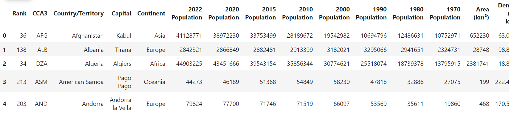
The dataset consists of 234 rows and 17 columns. The column names contain some special characters, which we must remove since the GridDB container does not allow column names to contain some of the special characters.
The script below replaces special characters in dataset columns with underscores and displays the data type of the columns.
dataset.columns = dataset.columns.str.replace('[^a-zA-Z0-9]', '_', regex=True)
dataset.dtypes
Output:
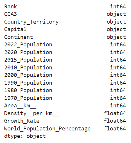
Verify the type of your input columns since you will need to map them to GridDB-compliant column types. For example, you will have to replace the object type with the string type before inserting the data into a GridDB container, as you will see later in the article.
We have preprocessed the dataset. The following steps include connecting with the GridDB and inserting our CSV data.
Note: You can directly plot data visualizations in Python using a Pandas dataframe. For the sake of demonstration in this blog, you will first insert the CSV data into a GridDB container, fetch the inserted data into a Pandas dataframe and then plot visualizations using the data retrieved from GridDB.
Creating a Connection with GridDB
To create a connection, you must create an object of the StoreFactory class, as shown in the script below.
Next, you must pass the GridDB host URL, the cluster name, and the user and password values to the factory object’s get_store() method. And that’s it.
To verify the connection is established, you can use the get_container() method to get any random container. If there is a connection issue, an exception will occur.
Run the script below. If you see the provided output, your connection is successful. If an exception occurs, verify your credentials, ensure the GridDB server is running, and check your configuration settings.
factory = griddb.StoreFactory.get_instance()

DB_HOST = "127.0.0.1:10001"
DB_CLUSTER = "myCluster"
DB_USER = "admin"
DB_PASS = "admin"

try:
    gridstore = factory.get_store(
        notification_member = DB_HOST,
        cluster_name = DB_CLUSTER,
        username = DB_USER,
        password = DB_PASS
    )

    container1 = gridstore.get_container("container1")
    if container1 == None:
        print("Container does not exist")
    print("Successfully connected to GridDB")

except griddb.GSException as e:
    for i in range(e.get_error_stack_size()):
        print("[", i, "]")
        print(e.get_error_code(i))
        print(e.get_location(i))
        print(e.get_message(i))
Output:
Container does not exist
Successfully connected to GridDB
Storing World Population Data in a GridDB Container
GridDB containers expect table columns to be in a specific data format. For further information, refer to GridDB data types.
To create a container, you first have to create an object of the ContainerInfo class and pass it four parameters: container name, container columns, container type, and a boolean value, which, if set to True treats the first column as the identity column.
The container columns must be a list of lists, each nested list containing a column name and the corresponding column type. Since our dataset does not have time-series data, we will set the container type to Collection.
The script below defines a map_pandas_dtype_to_griddb() function that maps the Pandas dataframe columns to GridDB column types. You can modify this method as per your requirements.
Next we create an object of the ContainerInfo class that stores our container information.
# see all GridDB data types: https://docs.griddb.net/architecture/data-model/#data-type

def map_pandas_dtype_to_griddb(dtype):
    if dtype == 'int64':
        return griddb.Type.LONG
    elif type == 'float64':
        return griddb.Type.FLOAT
    elif dtype == 'object':
        return griddb.Type.STRING
    # Add more column types if you want
    else:
        raise ValueError(f'Unsupported pandas type: {dtype}')

container_columns = []
for column_name, dtype in dataset.dtypes.items():
    griddb_dtype = map_pandas_dtype_to_griddb(str(dtype))
    container_columns.append([column_name, griddb_dtype])

container_info = griddb.ContainerInfo("PopulationStats",
                                      container_columns,
                                      griddb.ContainerType.COLLECTION, True)
Finally, to create a container object, call the put_container() method and pass it the container_info object you just created.
Finally, to insert records into your container, iterate through the rows in the input dataframe, convert each row to a Python list, and insert the list into the container object, as the following script demonstrates.
try:
    cont = grid store.put_container(container_info)
    for index, row in dataset.iterrows():
        cont.put(row.tolist())
    print("All rows have been successfully stored in the GridDB container.")

except griddb.GSException as e:
    for i in range(e.get_error_stack_size()):
        print("[", i, "]")
        print(e.get_error_code(i))
        print(e.get_location(i))
        print(e.get_message(i))
Output:
All rows have been successfully stored in the GridDB container.
The data has been successfully inserted into GridDB, as seen in the above message.
Next, you will learn how to read data from a GridDB container.
Retrieving World Population Data From a GridDB Container
In this section, we will fetch the world population data from the GridDB container and analyze it in the upcoming section using different visualizations.
The get_container() method fetches container data from GridDB. The query method of the container object allows you to execute SQL queries on this container.
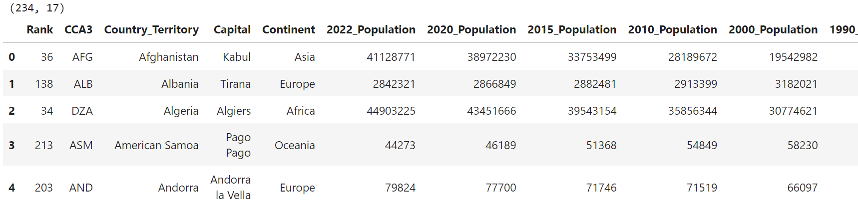
In the following script, we select all the data from the PopulationStats container using the fetch() method. Next, we retrieve all rows using the fetch_rows() method, which returns data as a Pandas dataframe.
population_container = gridstore.get_container("PopulationStats")
query = population_container.query("select *")
rs = query.fetch()
population_data = rs.fetch_rows()

print(population_data.shape)
population_data.head()
Output:
Visualizing World Population Data in Python using Data from GridDB
We have successfully retrieved the data we inserted into GridDB as a Pandas dataframe. Next, you can use this dataframe to analyze different aspects of the world population. You can plot different visualizations using any Python library, e.g., Pandas, Matplotlib, Seaborn, etc.
Let’s see some examples.
Analyzing World Population by Continent
You probably already know that Asia is the most populous continent in the world. But do you know what percentage of the global population Asia constitutes? You can visualize this information using a pie chart that sums the population of all countries by continent and then displays the percentage of the population for each continent.
The script below plots a pie chart of the world population grouped by continents.
population_by_continent = population_data.groupby('Continent')['2022_Population'].sum()

plt.figure(figsize=(6,6))
plt.pie(population_by_continent,
        labels=population_by_continent.index,
        autopct='%1.1f%%', startangle=140)
plt.title('World Population by Continent in 2022')
plt.show()
Output:
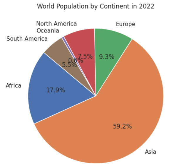
As we all know, the Asian continents account for around 59% of the total global population, followed by Africa and Europe.
Visualizing Top 10 Countries by World Population Percentage
Another interesting analysis is how much the top 10 most populous countries contribute to the global population.
To do so, you can create a bar graph that displays countries/territories and their corresponding world population percentages.
top_countries = population_data.sort_values('World_Population_Percentage', ascending=False).head(10)

plt.figure(figsize=(10, 8))
plt.barh(top_countries['Country_Territory'],
         top_countries['World_Population_Percentage'],
         color='skyblue')

plt.xlabel('% of world population')
plt.title('Top 10 Countries by World Population %')
plt.gca().invert_yaxis()  # Ensure the largest value is at the top
plt.show()
Output:
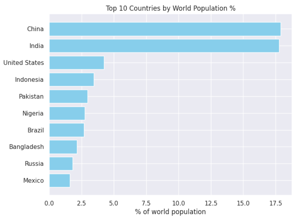
The above output shows that China and India each contribute around 17% of the global population. So, every third person on the globe is either an Indian or a Chinese.
Analyzing the Top 10 Most Dense Countries/Territories
In addition to total population, another exciting metric to analyze is population density, which refers to the population within a specific area (per kilometer square in our dataset).
This can tell us how congested a certain country or territory is. To retrieve this information, we can plot a bar graph that displays countries with the highest population density, as shown in the following script.
top_density_countries = population_data.nlargest(10, 'Density__per_km__')

plt.figure(figsize=(8, 6))
sns.barplot(x='Country_Territory', y='Density__per_km__', data=top_density_countries)
plt.xticks(rotation=45)
plt.title('Top 10 Countries/Territories by Population Density per Sq-km')
plt.xlabel('Country')
plt.ylabel('Density (per km²)')
plt.show()
Output:
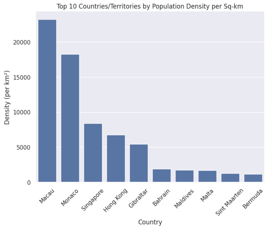
The output shows that Macau (a Chinese territory) has the highest population density (around 27 thousand) per square kilometer, followed by Monaco and Singapore.
Top 10 Most Densely Populated Countries in Europe and Asia
Let’s dig deeper and plot two bar plots for Asia and Europe, displaying the top ten countries/territories with the highest population density within these continents.
europe = population_data[population_data['Continent'] == 'Europe'].sort_values('Density__per_km__', ascending=False).head(10)
south_america = population_data[population_data['Continent'] == 'South America'].sort_values('Density__per_km__', ascending=False).head(10)

fig, axes = plt.subplots(1, 2, figsize=(14, 6))

axes[0].barh(europe['Country_Territory'], europe['Density__per_km__'], color='skyblue')
axes[0].set_title('Top 10 Densely Populated Countries/Territories in Europe')
axes[0].invert_yaxis()

axes[1].barh(south_america['Country_Territory'], south_america['Density__per_km__'], color='lightgreen')
axes[1].set_title('Top 10 Densely Populated Countries/Territories in South America')
axes[1].invert_yaxis()

plt.tight_layout()
plt.show()
Output:
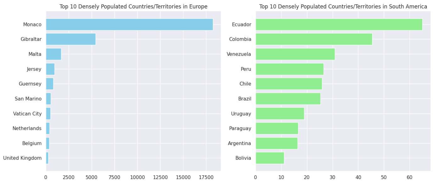
As you can see, Monaco is the most densely populated territory in Europe, while Ecuador is the most densely populated country in South America.
Population Growth from 1970 to 2022 for Top 10 Most Populous Countries
Another exciting aspect of the world population is the population growth rate. This can help identify countries that need to control their population.
For example, using a line plot, the following script shows the population growth rates for the top ten most populous countries from 1970 to 2022.
top_countries = population_data.sort_values(by='World_Population_Percentage', ascending=False).head(10)

data = pd.melt(top_countries,
               id_vars=['Country_Territory'],
               value_vars=['1970_Population', '1980_Population', '1990_Population', '2000_Population', '2010_Population', '2015_Population', '2020_Population', '2022_Population'],
               var_name='Year',
               value_name='Population')

data['Year'] = data['Year'].str.extract('(d+)').astype(int)


plt.figure(figsize=(9, 6))
sns.line plot(x='Year',
             y='Population',
             hue='Country_Territory',
             data=data, marker='o')

plt.title('Population Growth from 1970 to 2022 for Top 10 Most Populous Countries')
plt.legend(title='Country')
plt.show()
Output:
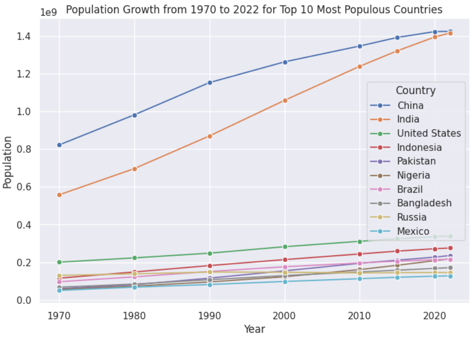
The above output shows that the population difference between India and China was around 200 million in 1970, which has narrowed to almost negligible by the end of 2022.
These are some of the interesting observations from the world population dataset. You can further analyze and visualize the dataset using the same techniques to extract more exciting information.
Updating GridDB Data Using SQL UPDATE QUERY
In addition to inserting and retrieving data, GridDB allows you to update existing data easily. To do so, select the row and column you want to update and assign the updated value to the selected cell.
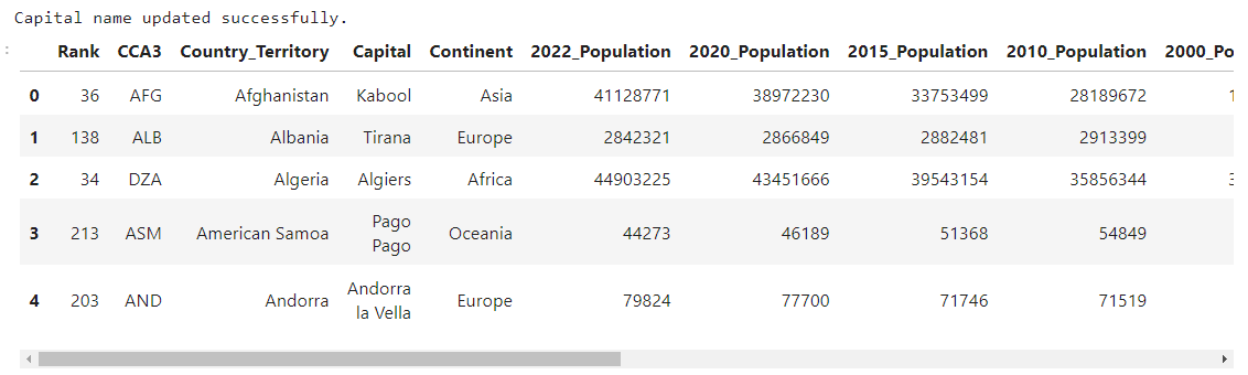
For example, you can use the following script to update the value in the Capital column where the Country_Territory column contains Afghanistan. The script first selects the row where the Country_Territory column equals Afghanistan and then selects the index of the Capital column using our Pandas dataframe. The script then updates the cell value using the update() method. Finally, the container’s commit() function commits the change to the container in the GridDB.
population_container.set_auto_commit(False)
query = population_container.query("SELECT * WHERE Country_Territory = 'Afghanistan'")
rs = query.fetch(True)

if rs.has_next():
    data = rs.next()
    capital_index = population_data.columns.get_loc('Capital')

    data[capital_index] = 'Kabool'
    rs.update(data)

population_container.commit()
print("Capital name updated successfully.")

query = population_container.query("select *")
rs = query.fetch()
population_data = rs.fetch_rows()
population_data.head()
Output:
Deleting GridDB Data Using SQL DELETE QUERY
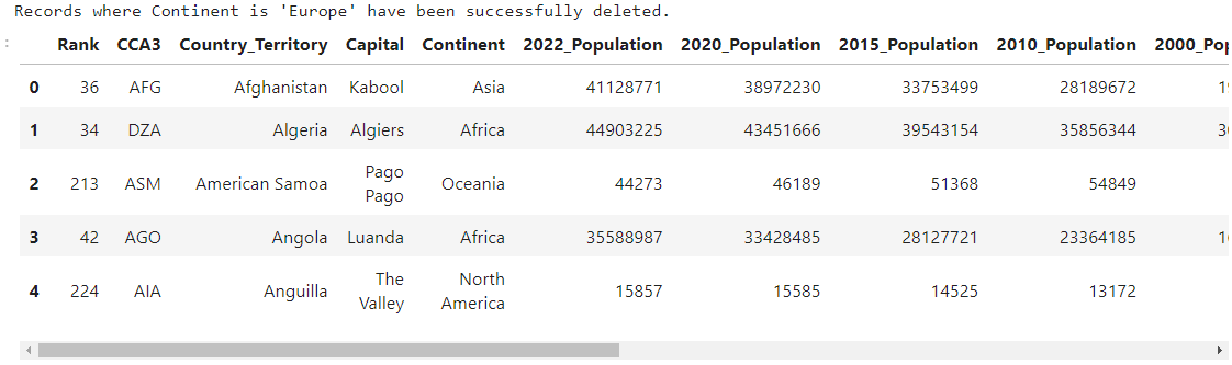
Similarly, you can use the remove() method of the object returned by the fetch() query to remove a row from a GridDB container. The following script demonstrates removing all rows where the Continent column contains the value Europe.
population_container.set_auto_commit(False)

query = population_container.query("SELECT * WHERE Continent = 'Europe'")

rs = query.fetch(True)

while rs.has_next():
    data = rs.next()
    rs.remove()


population_container.commit()
print("Records where Continent is 'Europe' have been successfully deleted.")

query = population_container.query("select *")
rs = query.fetch()
population_data = rs.fetch_rows()
population_data.head()
Output:
Conclusion
In this article, you analyze the world population dataset using Python with GridDB as the database. The analysis revealed interesting information about the world population.In addition, you learned how to connect Python to the GridDB database. You saw how to insert CSV data into a GridDB container and then fetch data from a GridDB container into a Pandas dataframe.
GridDB is a highly scaleable open-source database that allows you to efficiently store and retrieve all varieties of data using NoSQL and traditional SQL queries. GridDB database is highly recommended for managing IoT and time-series datasets.
You can find the Jupyter Notebook for this blog on Github.
If you have any questions or queries related to GridDB, create a Stackoverflow post. Remember to use the griddb tag so our engineers can respond quickly.
If you have any questions about the blog, please create a Stack Overflow post here https://stackoverflow.com/questions/ask?tags=griddb .
Make sure that you use the “griddb” tag so our engineers can quickly reply to your questions.