
This article explains how to build a time series forecasting model using TensorFlow Keras and GridDB. We will retrieve historical stock market data from Yahoo Finance, store it in a GridDB time series container, and use it to train a TensorFlow Keras transformer model for time series forecasting.
GridDB is a robust NoSQL database designed for handling large volumes of real-time data with exceptional efficiency. Its advanced in-memory processing and time series data management features make it an ideal choice for big data and IoT applications, including financial forecasting and real-time analytics.
Prerequisites
To run the code in this article, you will need the following libraries:
- GridDB C Client
- GridDB Python client
Follow the instructions on the GridDB Python Package Index (Pypi) page to install these clients.
You will also need to install TensorFlow, yfinance, Numpy, Pandas, and Matplotlib libraries.
The scripts below will help you install and import the necessary libraries for running the code in this article.
pip install yfinance
python3 -m pip install tensorflow[and-cuda]
import os
import absl.logging
os.environ['TF_CPP_MIN_LOG_LEVEL'] = '3'
os.environ['TF_ENABLE_ONEDNN_OPTS'] = '0'
absl.logging.set_verbosity(absl.logging.ERROR)
os.environ['CUDA_VISIBLE_DEVICES'] = '-1'
import yfinance as yf
import pandas as pd
import griddb_python as griddb
import numpy as np
import tensorflow as tf
from tensorflow import keras
from tensorflow.keras import layers
from tensorflow.keras.utils import disable_interactive_logging
import matplotlib.pyplot as plt
from sklearn.preprocessing import MinMaxScalerInserting Stock Market Data into GridDB
We will use stock market data from Yahoo Finance to train our time series forecasting model.
In this section, you will see how to fetch stock market data from Yahoo Finance, create a connection with GridDB, and insert the Yahoo finance data into a GridDB container.
Fetch Data from Yahoo Finance
The yfinance.download() method allows you to retrieve data from Yahoo Finance into a Pandas dataframe.
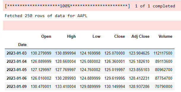
In the script below we retrieve Apple’s stock prices for the full year of 2023:
ticker = "AAPL"
start_date = "2023-01-01"
end_date = "2023-12-31"
data = yf.download(ticker, start=start_date, end=end_date)
print(f"Fetched {len(data)} rows of data for {ticker}")
data.head()
Output:
Connect to GridDB
To connect to GridDB you need to call the griddb.StoreFactory.get_instance() method to get a GridDB factory instance object.
Next, you need to create a GridDB factory store object using the get_store() method. You will need to pass your GridDB host name, cluster, name and user and password to the get_store() method. Finally, you can test your connection by randomly retrieve a GridDB container using the get_container() method.
The following script shows how to connect to GridDB and test your GridB connection:
# GridDB connection details
DB_HOST = "127.0.0.1:10001"
DB_CLUSTER = "myCluster"
DB_USER = "admin"
DB_PASS = "admin"

# creating a connection

factory = griddb.StoreFactory.get_instance()

try:
   gridstore = factory.get_store(
       notification_member = DB_HOST,
       cluster_name = DB_CLUSTER,
       username = DB_USER,
       password = DB_PASS
   )

   container1 = gridstore.get_container("container1")
   if container1 == None:
       print("Container does not exist")
   print("Successfully connected to GridDB")

except griddb.GSException as e:
   for i in range(e.get_error_stack_size()):
       print("[", i, "]")
       print(e.get_error_code(i))
       print(e.get_location(i))
       print(e.get_message(i))
Output:
Container does not exist
Successfully connected to GridDB
Create Container for Stock Data in GridDB
A GridDB container is a fundamental data structure in used for storing and managing data in GridDB.
We will store the Yahoo Finance data we retrieved in a time series type container.
To create a container you first need to call the ContainerInfo() method and pass it the container name, a list of lists containing data columns and types, and the container type which in our case will be griddb.ContainerType.TIME_SERIES.
Next, call the put_container() method and pass it as a parameter the container info object you previously created.
The script below shows how to create the AAPL_stock_data container in GridDB.
container_name = f"{ticker}_stock_data"
column_info = [
    ["Timestamp", griddb.Type.TIMESTAMP],
    ["Open", griddb.Type.DOUBLE],
    ["High", griddb.Type.DOUBLE],
    ["Low", griddb.Type.DOUBLE],
    ["Close", griddb.Type.DOUBLE],
    ["Volume", griddb.Type.LONG]
]
container_info = griddb.ContainerInfo(container_name, column_info, griddb.ContainerType.TIME_SERIES)

try:
    gridstore.put_container(container_info)
    container = gridstore.get_container(container_name)
    if container is None:
        print(f"Failed to create or retrieve container: {container_name}")
    else:
        print(f"Successfully created and retrieved container: {container_name}")
except griddb.GSException as e:
    print(f"Error creating or retrieving container {container_name}:")
    for i in range(e.get_error_stack_size()):
        print(f"[{i}]")
        print(f"Error code: {e.get_error_code(i)}")
        print(f"Location: {e.get_location(i)}")
        print(f"Message: {e.get_message(i)}")
Output:
Successfully created and retrieved container: AAPL_stock_dataInsert Data into GridDB Container
The last step is to insert the Yahoo Finance data from the Pandas DataFrame into the GridDB container you created in the previous script.
To do so, you can iterate through all the rows of a Pandas DataFrame, call the container’s put() method and pass it the data you want to store in the container.
The script below shows how to store Yahoo Finance Data in a GridDB container.
try:
    for index, row in data.iterrows():
        container.put([index.to_pydatetime(), row['Open'], row['High'], row['Low'], row['Close'], int(row['Volume'])])
    print(f"Successfully inserted {len(data)} rows of data into {container_name}")
except griddb.GSException as e:
    print(f"Error inserting data into container {container_name}:")
    for i in range(e.get_error_stack_size()):
        print(f"[{i}]")
        print(f"Error code: {e.get_error_code(i)}")
        print(f"Location: {e.get_location(i)}")
        print(f"Message: {e.get_message(i)}")
Output:
Successfully inserted 250 rows of data into AAPL_stock_dataCreating a Stock Market Forecasting Model Using TensorFlow Keras
We have now Successfully stored our time series stock market data in GriDB, next we will train a TensorFlow Keras model for time series forecasting.
Retrieving Data from GridDB
First we will retrieve data from our GridDB container and store it in a Pandas DataFrame.
To do so, call the get_container() method and pass to it the name of the container you want to retrieve.
Next, call SELECT * query on the container using the query() method.
Call the fetch() method to run the query and finally the fetch_rows() function to store returned records in a Pandas DataFrame.
def retrieve_data_from_griddb(container_name):
try:
stock_data_container = gridstore.get_container(container_name)
# Query all data from the container
query = stock_data_container.query("select *")
rs = query.fetch() # Adjust the number based on your data size
data = rs.fetch_rows()
data .set_index("Timestamp", inplace=True)
return data
except griddb.GSException as e:
print(f"Error retrieving data from GridDB: {e.get_message()}")
return none
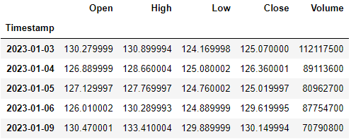
stock_data = retrieve_data_from_griddb("AAPL_stock_data")
stock_data.head()
Output:
Data Preprocessing for TensorFlow Keras Transformer Model
We will use a Transformer model from TensorFlow Keras for time series forecasting in this article. You can also use a long short term memory (LSTM) or one-dimensional convolutional neural networks (1D-CNN) as well. However, transformers, being the state of the art are likely to outperform the other models.
We will use the Open and Volume stock prices for the last seven days to predict the Open stock price for the next day.
To do so, we will divide our data into into feature (X) and labels (y) set, and the into training (80%) and test(20%) sets. We will also normalize our data since deep learning models are known to work better with the normalized data.
The following script preprocesses and normalizes the dataset.
features = ['Open', 'Volume']
data = stock_data[features].values

# Initialize the scaler
scaler = MinMaxScaler(feature_range=(0, 1))

# Fit the scaler to the data and transform
data_normalized = scaler.fit_transform(data)

# Create sequences
def create_sequences(data, seq_length):
    X, y = [], []
    for i in range(len(data) - seq_length):
        X.append(data[i:(i + seq_length), :])
        y.append(data[i + seq_length, 0])  # Predicting next day's Open price
    return np.array(X), np.array(y)


seq_length = 7 # stock prices of last 7 days
X, y = create_sequences(data_normalized, seq_length)

# Split the data into training and testing sets
split = int(0.8 * len(X))
X_train, X_test = X[:split], X[split:]
y_train, y_test = y[:split], y[split:]
Creating a TensorFlow Keras Transformer Model
Next, we will define our transformer model architecture. Our model will consist of a multiheaded attention layer, followed by two 1-D convolutional neural network layers. We will also add dropout and layer normalization to avoid overfitting. You can modify the model architecture if you want.
# Define the Transformer block
def transformer_encoder(inputs, head_size, num_heads, ff_dim, dropout=0):
    # Attention and Normalization
    x = layers.MultiHeadAttention(
        key_dim=head_size, num_heads=num_heads, dropout=dropout
    )(inputs, inputs)
    x = layers.Dropout(dropout)(x)
    x = layers.LayerNormalization(epsilon=1e-6)(x)
    res = x + inputs

    # Feed Forward Part
    x = layers.Conv1D(filters=ff_dim, kernel_size=1, activation="relu")(res)
    x = layers.Dropout(dropout)(x)
    x = layers.Conv1D(filters=inputs.shape[-1], kernel_size=1)(x)
    x = layers.LayerNormalization(epsilon=1e-6)(x)
    return x + res
=Subsequently, we will define the build_model() method that builds our model. The model takes our data features and labels as inputs, pass the data through transformer model we just defined. The output of the transformer model is passed through a global average pooling layer, followed by three dense layers to get the final model output.
# Build the model
def build_model(
    input_shape,
    head_size,
    num_heads,
    ff_dim,
    num_transformer_blocks,
    mlp_units,
    dropout=0,
    mlp_dropout=0,
):
    inputs = keras.Input(shape=input_shape)
    x = inputs
    for _ in range(num_transformer_blocks):
        x = transformer_encoder(x, head_size, num_heads, ff_dim, dropout)

    x = layers.GlobalAveragePooling1D(data_format="channels_first")(x)
    for dim in mlp_units:
        x = layers.Dense(dim, activation="relu")(x)
        x = layers.Dropout(mlp_dropout)(x)
    outputs = layers.Dense(1)(x)
    return keras.Model(inputs, outputs)
Next, we pass the model configurations to the build_model() function and get the model object back from the function. We call the compile() method to compile the model.
# Create the model
input_shape = X_train.shape[1:]
model = build_model(
    input_shape,
    head_size=256,
    num_heads=4,
    ff_dim=4,
    num_transformer_blocks=4,
    mlp_units=[128],
    mlp_dropout=0.4,
    dropout=0.25,
)
# Compile the model
model.compile(
    optimizer=keras.optimizers.Adam(learning_rate=1e-4),
    loss="mse",
    metrics=["mae"]
)
Next, we define call backs for early stopping, storing the best model weights, and reducing the learning rate.
Finally, we call the fit() method an pass it our training data to start model training.
# Define callbacks
callbacks = [
    keras.callbacks.EarlyStopping(patience=10, restore_best_weights=True),
    keras.callbacks.ReduceLROnPlateau(factor=0.5, patience=5, min_lr=1e-6),
]

# Train the model
history = model.fit(
    X_train,
    y_train,
    validation_split=0.2,
    epochs=100,
    batch_size=32,
    callbacks=callbacks,
)
Output:
![]()
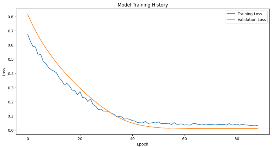
The script below shows the training and validation losses for our model. The curves show that our model is not overfitting.
plt.figure(figsize=(12, 6))
plt.plot(history.history['loss'], label='Training Loss')
plt.plot(history.history['val_loss'], label='Validation Loss')
plt.title('Model Training History')
plt.ylabel('Loss')
plt.xlabel('Epoch')
plt.legend()
plt.show()
Output:
Evaluating the Model Performance
Let’s evaluate our model’s performance on the training and test sets.
The output of the following script shows that we receive a mean absolute error score of 0.1596 which is greater than 0.0788. This shows that our model is overfitting on training set.
Next, we will plot the actual and predicted stock prices side-by-side on a line plot. It is important to note that we have to inverse the effect of data scaling that we did during the data preprocessing step.
The following script also does that.
test_loss, test_mae = model.evaluate(X_test, y_test)
print(f"Test MAE: {test_mae:.4f}")

# When making predictions and inverse transforming:
train_predictions = model.predict(X_train)
test_predictions = model.predict(X_test)

# Inverse transform predictions (for Open price only)
train_predictions = scaler.inverse_transform(np.column_stack((train_predictions, np.zeros_like(train_predictions))))[:, 0]
test_predictions = scaler.inverse_transform(np.column_stack((test_predictions, np.zeros_like(test_predictions))))[:, 0]

# Inverse transform actual values
y_train_actual = scaler.inverse_transform(np.column_stack((y_train.reshape(-1, 1), np.zeros_like(y_train.reshape(-1, 1)))))[:, 0]
y_test_actual = scaler.inverse_transform(np.column_stack((y_test.reshape(-1, 1), np.zeros_like(y_test.reshape(-1, 1)))))[:, 0]
Output:
Test MAE: 0.1596Finally, the script below plots the actual stock prices for the training set, and the actual and predicted stock prices for the test set.
# Get the actual prices for the entire dataset
y_actual = np.concatenate([y_train_actual, y_test_actual])

# Create a date range for the entire dataset
full_date_range = pd.date_range(start=stock_data.index[seq_length], periods=len(y_actual), freq='B')

# Get the date range for the test set
test_date_range = full_date_range[-len(y_test_actual):]

# Plot results
plt.figure(figsize=(20, 10))

# Plot the entire actual price series
plt.plot(full_date_range, y_actual, label='Actual', color='blue')

# Plot only the test predictions
plt.plot(test_date_range, test_predictions, label='Predicted (Test Set)', color='red', linestyle='--')

# Add a vertical line to indicate the start of the test set
split_date = full_date_range[-len(y_test_actual)]
plt.axvline(x=split_date, color='green', linestyle='--', label='Test Set Start')

plt.title('Stock Open Price - Actual vs Predicted (Test Set)', fontsize=20)
plt.xlabel('Date', fontsize=16)
plt.ylabel('Open Price', fontsize=16)
plt.legend(fontsize=14)
plt.grid(True, which='both', linestyle='--', linewidth=0.5)

# Rotate and align the tick labels so they look better
plt.gcf().autofmt_xdate()


# Show the plot
plt.show()
Output:
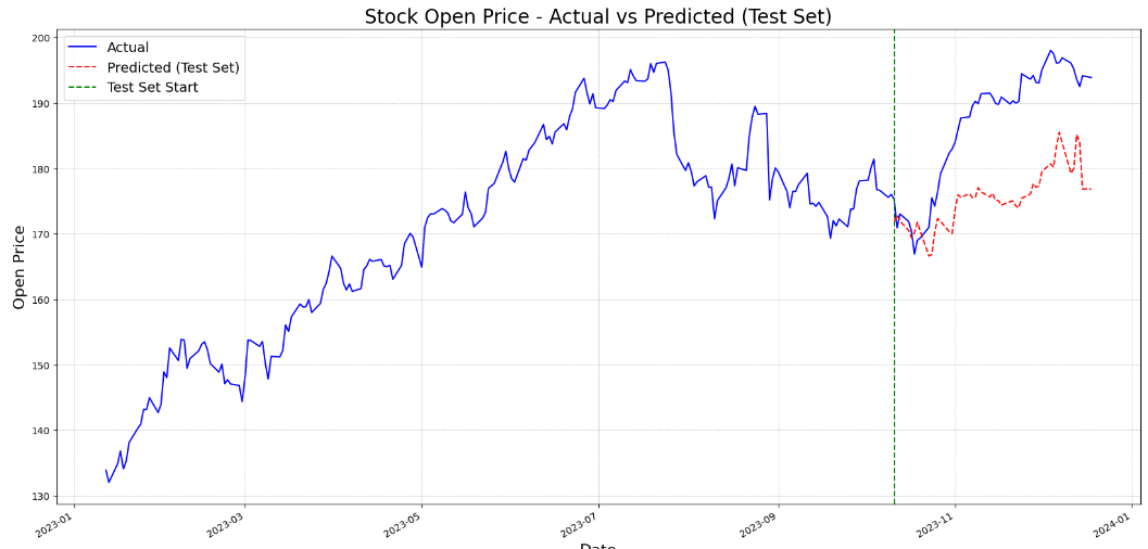
From the above output, you can see that model predictions are quite close to the actual stock prices. The model also captures the bullish and bearish trend.
Conclusion
In this article, you learned how to create a TensorFlow Keras model for time series forecasting using data from GridDB. We explored how to connect to GridDB, insert financial data into a time series container, and retrieve it for further processing. We also demonstrated how to build a Transformer-based neural network model for predicting stock prices. You can use the code in this article for developing any time series forecasting model using GridDB time series data.
GridDB is a highly efficient NoSQL database, optimized for handling large-scale time series data, which makes it ideal for applications like financial forecasting and real-time analytics. Using TensorFlow’s advanced deep learning and AI capabilities and GridDB’s powerful data management system, you can build scalable and performant forecasting models.
You can find the complete code for this blog on my GridDB Blogs GitHub repository. For any questions or issues related to GridDB, feel free to reach out on Stack Overflow using the griddb tag to get prompt response from our engineers.
Please note: This article is for educational purposes only and does not serve as financial or stock trading advice.