Data Analysis aims to extract useful information from data and then aids the decision making process. However, the raw data we get from external sources, be it mobile devices or sensors, has many outliers. Moreover, the data may be high dimensional, so it becomes hard to interpret the data's summary statistics. As a result, nowadays, data analysis is the umbrella term for the process of getting raw data to getting human interpretable results. Thus, data analysis consists of data cleaning, transforming and modelling such that meaningful information can be extracted from it.
The most crucial precursor of a good data analysis system has a reliable database. Our database should be scalable, and we should be able to query large datasets easily from it. One such modern database that allows for all these functionalities is GridDB. GridDB is a high performance and can easily be integrated with many programming languages. In this post, we will analyze some data with python and GridDB. As there are many types of analyses we can do, we will focus on a random forest model in this post.
GridDB setup
This video has the setup guide for the GridDB python client.
Python libraries
We will use python 3.6 and pandas to do our analysis.
To install libraries we use the following command:
pip install pandas
pip install scikit-learn
pip install plotly
pip install matplotlib
import libraries
import pandas as pd
import matplotlib.pyplot as plt
import plotly.graph_objs as go
from plotly.subplots import make_subplots
from sklearn.model_selection import train_test_split,cross_val_score
from sklearn.ensemble import RandomForestClassifier
from sklearn.metrics import f1_score as f1
Data Collection
GridDB provides an excellent interface to access data. The GridDB python client blog goes into great detail to link a GridDB database and push all the data to a pandas data frame.
For this analysis we will use credit card data to predict attrition or churn. The data can be found here.
We can set up GridDB as our database by instantiating the container and dumbing all the data into a pandas dataframe.
import griddb_python as griddb
# Initialize container
gridstore = factory.get_store(host= host, port=port,
            cluster_name=cluster_name, username=uname,
            password=pwd)

conInfo = griddb.ContainerInfo("attrition",
                    [["CLIENTNUM", griddb.Type.LONG],
                    ["Gender",griddb.Type.STRING],
              .... #for all 23 variables
                    griddb.ContainerType.COLLECTION, True)

cont = gridstore.put_container(conInfo)
cont.create_index("CLIENTNUM", griddb.IndexType.DEFAULT)
We can retrive data from GridDB using the following SQL query:
query = cont.query("select *")
The data analysis pipeline has the following steps:
- Data exploration: We first run some summary statistics on the various variables we have and try to understand the correlation with the dependent variable, i.e. survival. We also clean the dataset to remove outliers, if any.
- Feature Engineering: We will then select the features that can be used for modelling. We can create new features either from existing data or open-source resources.
- Modelling: We then use a machine learning model, random forest, in our case. We would first split the data into a test set and a training set. Typically we train the model on the training data and evaluate it on the test set. Sometimes we either have a validation set or do cross-validation to tune the hyperparameters of the model.
- Evaluation: Finally, we will use the model for prediction and analyze its performance.
Data Collection and Exploration
We load the data using pandas. We remove the last two columns as they are the results of a different classifier.
data = pd.read_csv('/kaggle/input/credit-card-customers/BankChurners.csv')
data = data[data.columns[:-2]]
We first create summary statistics of some of the variables. Ideally, we would check every variable, but for brevity, we showcase a few important ones.
Attrition_Flag:
attdata = data.groupby(['Attrition_Flag']).count()[["CLIENTNUM"]].reset_index()
attdata['percentage'] = attdata['CLIENTNUM']/attdata['CLIENTNUM'].sum()
attdata[attdata.Attrition_Flag == "Attrited Customer"]| CLIENTNUM | percentage |
|---|---|
| 1627 | 0.16066 |
We have an attrition of about 16%.
Demographic Variables
Gender
genderdata = data.groupby(['Gender']).count()[["CLIENTNUM"]].reset_index()
genderdata['percentage'] = genderdata['CLIENTNUM']/genderdata['CLIENTNUM'].sum()
genderdata[genderdata.Gender == "F"]| CLIENTNUM | percentage |
|---|---|
| 5358 | 0.529081 |
We see that there are 52.9% females. But the difference in the genders is not that significant.
Education
data.groupby(['Education_Level']).count()[["CLIENTNUM"]].reset_index()
Education_Level
| Type | Number |
|---|---|
| College | 1013 |
| Doctorate | 451 |
| Graduate | 3128 |
| High School | 2013 |
| Post-Graduate | 516 |
| Uneducated | 1487 |
| Unknown | 1519 |
We see about 70% of the customers are educated.
Income_Category
data.groupby(['Income_Category']).count()[["CLIENTNUM"]].reset_index()
| Income_Category | Number |
|---|---|
| $120K + | 727 |
| 40k− 60k | 1790 |
| 60k− *80K | 1402 |
| Less than $40k | 3561 |
| Unknown | 1112 |
We see that most people earn less than $40k.
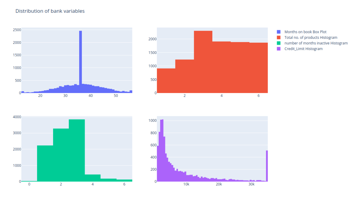
Bank variables
We will draw histograms for Months_on_book, 'Total_Relationship_Count',
'Months_Inactive_12_mon' and 'Credit_Limit'
fig = make_subplots(rows=2, cols=2)
tr1=go.Histogram(x=data['Months_on_book'],name='Months on book Box Plot')
tr2=go.Histogram(x=data['Total_Relationship_Count'],name='Total no. of products Histogram')
tr3=go.Histogram(x=data['Months_Inactive_12_mon'],name='number of months inactive Histogram')
tr4=go.Histogram(x=data['Credit_Limit'],name='Credit_Limit Histogram')

fig.add_trace(tr1,row=1,col=1)
fig.add_trace(tr2,row=1,col=2)
fig.add_trace(tr3,row=2,col=1)
fig.add_trace(tr4,row=2,col=2)

fig.update_layout(height=700, width=1200, title_text="Distribution of bank variables")
fig.show()
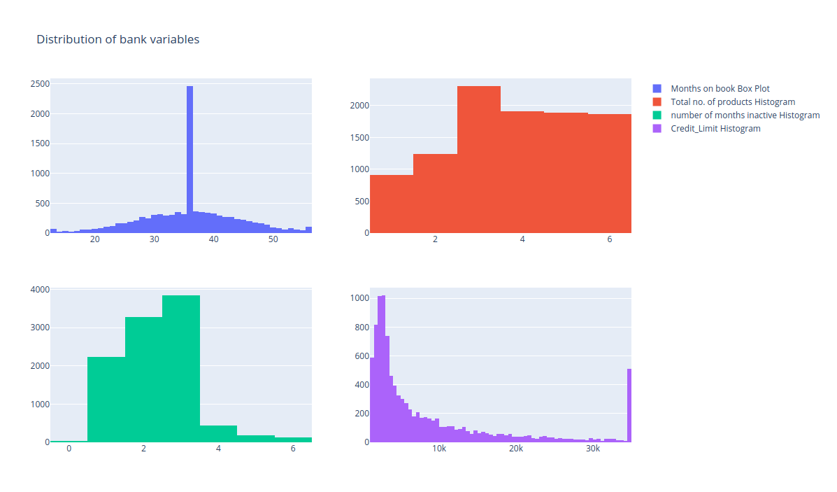
We see that the distribution of the total number of products is mostly uniform so ideally this variable can be removed from our analysis. Other variables show a lot of variation so we can keep them.
Card_Category
data.groupby(['Card_Category']).count()[["CLIENTNUM"]].reset_index()
| Card_Category | Total |
|---|---|
| Blue | 9496 |
| Gold | 116 |
| Platinum | 20 |
| Silver | 555 |
We see that most customers use Blue so we can ignore this variable as well.
Feature Engineering
We can ignore the client number for this analysis. However, if the bank had more data source then the client number could be used to match different datasets.
The attrition flag is our dependent variable as we want to predict attrition. We will code this as a 0,1 variable.
Next, we create dummy variables. Dummy variables essentially encode the variables of one category. We will leave one category out. Otherwise, we'll face the issue of collinearity. We create dummy variables from the Demographic variable. This is also known as Hot-One Encoding.
- Education_Levels
- Income
- Marital status
data.Attrition_Flag = data.Attrition_Flag.replace({'Attrited Customer':1,'Existing Customer':0})
data.Gender = data.Gender.replace({'F':1,'M':0})
data = pd.concat([data,pd.get_dummies(data['Education_Level']).drop(columns=['Unknown'])],axis=1)
data = pd.concat([data,pd.get_dummies(data['Income_Category']).drop(columns=['Unknown'])],axis=1)
data = pd.concat([data,pd.get_dummies(data['Marital_Status']).drop(columns=['Unknown'])],axis=1)

data.drop(columns = ['Education_Level','Income_Category','Marital_Status','Card_Category','CLIENTNUM', 'Card_Category'],inplace=True, errors = "ignore")
Data Modelling
Next we run a simple random forest model with 100 trees after splitting the data into test and train.
X_features = ['Customer_Age', 'Gender', 'Dependent_count',
'Months_on_book', 'Total_Relationship_Count', 'Months_Inactive_12_mon',
'Contcts_Count_12_mon', 'Credit_Limit', 'Total_Revolving_Bal',
'Avg_Open_To_Buy', 'Total_Amt_Chng_Q4_Q1', 'Total_Trans_Amt',
'Total_Trans_Ct', 'Total_Ct_Chng_Q4_Q1', 'Avg_Utilization_Ratio',
'College', 'Doctorate', 'Graduate', 'High School', 'Post-Graduate',
'Uneducated', '$120K +', '$40K - $60K', '$60K - $80K', '$80K - $120K',
'Less than $40K', 'Divorced', 'Married', 'Single']


X = data[X_features]
y = data['Attrition_Flag']
train_x,test_x,train_y,test_y = train_test_split(X,y,random_state=42)

rf = RandomForestClassifier(n_estimators = 100, random_state = 42)
rf.fit(train_x,train_y)
Evaluation
We find the F1 score on prediction. F1 is defined as the harmonic mean of precision and recall.
rf_prediction = rf_pipe.predict(test_x)
print('F1 Score of Random Forest Model On Test Set {}'.format(f1(rf_prediction,test_y)))
We can also get relative variable importances from the random forest model.
importances = rf.feature_importances_
indices = np.argsort(importances)
plt.title('Feature Importances')
plt.barh(range(len(indices)), importances[indices], color='b', align='center')
plt.yticks(range(len(indices)), [X_features[i] for i in indices])
plt.xlabel('Relative Importance')
plt.show()
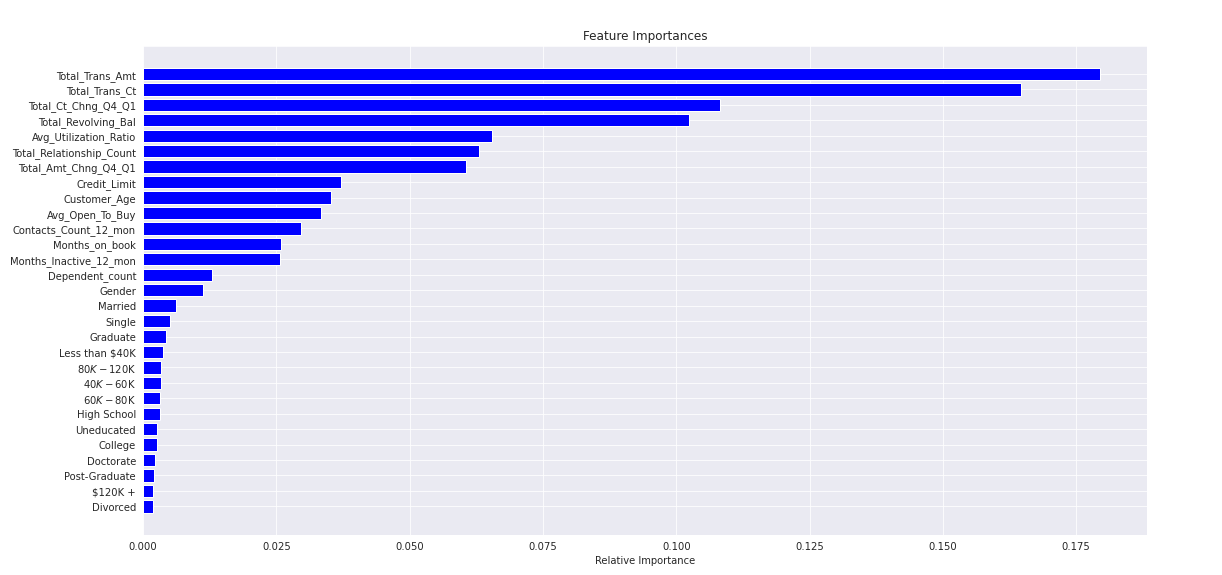
We see that the total transaction amount is the most important variable.
Conclusion
In this post we learned the basics of data analysis and predictive modelling using python and GridDB.