Bridging Python and GridDB CLI to validate Air Quality Sensor Outputs
GridDB is an open-source database designed for high-performance computing and analytics. While it is optimized for time-series data and IoT applications, it also offers support for general-purpose data storage similar to relational database tables. This flexibility allows developers to choose the best format depending upon the data they're working with — whether it's event logs, sensor and device metrics, or transactional records.
In this article, we begin by exploring the various methods available to connect to GridDB Cloud (Refer to section Methods to Connect to GridDB). We then delve deeper into the usage of the GridDB Cloud CLI tool. The The GridDB Cloud CLI Tool is a command line interface that helps interact with GridDB Cloud to seamlessly connect to the Cloud instance, create containers, ingest and query data. Let's learn more about this tool using a public dataset named 'Air Quality Data' from the UCI Machine Learning Laboratory (More information on the data is available in the section Importing a Public Dataset into Python). Click here to access the Quick Start Guide of GridDB Cloud .
Importing Libraries
# --- Data handling & processing ---
import pandas as pd
import base64
import requests
import os
import json
import http.client
from io import StringIO
import yaml  # To set up credentials in a YAML file

# --- Display utilities ---
from IPython.display import Image, display, HTML

# --- Visualization libraries ---
import matplotlib.pyplot as plt
from matplotlib.colors import LinearSegmentedColormap
import seaborn as sns
import plotly.express as px
import plotly.graph_objects as go

# --- External process handling ---
import subprocess

# --- Dataset access (UCI ML Repository) Library to download UCI Machine Learning Laboratory's Air Quality Dataset ---
import ucimlrepo
from ucimlrepo import fetch_ucirepo
Methods to Connect to GridDB
There are various methods to connect to GridDB, each catering to a different scenario and a different use case. Below is a list of the same -
- JayDeBeApi
- GridDB Cloud
- GridDB WebAPI (RESTful API)
- GridDB Native Clients
- Community CLI for GridDB Cloud (griddb-cloud-cli)
| Method | Type | Usage | Example |
|---|---|---|---|
| JayDeBeApi | Python via JDBC | Connect GridDB to Python using Java JDBC driver |
|
| GridDB Cloud | Managed Cloud Platform | Web-based GridDB with quick provisioning via GUI or API tokens |
|
| WebAPI (REST API) | RESTful HTTP | Send HTTP requests to interact with GridDB containers and rows |
|
| Native Clients | Official Language SDKs | Connect using language-specific libraries (Python, Java, C, etc.) |
|
| griddb-cloud-cli | Community CLI | Command-line tool that interfaces with GridDB Cloud's REST API |
|
Setting Up GridDB-Cloud-CLI on Your Machine
Step 1: Start by cloning the repository -
- git clone https://github.com/Imisrael/griddb-cloud-cli.git
- cd griddb-cloud-cli
Step 2: Ensure you have Go installed on your machine. You can download it from the official Go website: https://go.dev/dl/
After installation, open a new Command Prompt window and run:
- go version
Step 3: Go ahead and build the tool -
- cd griddb-cloud-cli
- go build -o griddb-cloud-cli main.go
Finally, run the below command.
go build -o griddb-cloud-cli main.goThis will generate an executable named griddb-cloud-cli in the current directory.
Configuring Access to GridDB Cloud with a YAML File
According to the README in the GridDB Cloud CLI GitHub repository, you would need to create a YAML file containing your user credentials and the cloud URL.
Below is the method to create it using Python:
config = {
    "cloud_url": "https://[host]:[port]/griddb/v2/[clustername]/dbs/[database_name]/",
    "cloud_username": "XXXXX",
    "cloud_pass": "XXXXX"
}

yaml_path = os.path.expanduser("~/.griddb.yaml")
with open(yaml_path, 'w') as file:
    yaml.dump(config, file)
Running the Binary Executable
Run the command below to run the binary executable -
.\griddb-cloud-cli.exe --help
If you get the error ''..\griddb-cloud-cli' is not recognized as an internal or external command,
operable program or batch file.' while running the above command, try renaming the file with the extension '.exe'
rename griddb-cloud-cli griddb-cloud-cli.exe
Checking the Connection to GridDB Cloud
Make sure you have your IP Address whitelisted on GridDB Cloud in the 'Network Access' tab.
result = subprocess.run(
    ["C:\\Users\\...\\griddb-cloud-cli.exe", "checkConnection"],
    stdout=subprocess.PIPE,
    stderr=subprocess.PIPE,
    text=True  # ensures output is string instead of bytes
)

print("Output:", result.stdout)
print("Errorifany:", result.stderr)
print("Return Code:", result.returncode)
Output: 200 OK

Errorifany:
Return Code: 0
Importing a Public Dataset into Python
For this purpose, we will use the Air Quality Dataset for our analysis. More information on this dataset is available here. The data can be imported directly into Python using the library ucimlrepo.
# fetch dataset
dataset = fetch_ucirepo(id=360)
df = pd.concat([dataset.data.features, dataset.data.targets], axis=1)
#print(df.head())

#Creating a datetime column for use in a container
df['datetime'] = pd.to_datetime(df['Date'] + ' ' + df['Time'])


# Renaming columns
df = df.rename(columns={
    'CO(GT)': 'co_gt',
    'PT08.S1(CO)': 'pt08_s1_co',
    'NMHC(GT)': 'nmhc_gt',
    'C6H6(GT)': 'c6h6_gt',
    'PT08.S2(NMHC)': 'pt08_s2_nmhc',
    'NOx(GT)': 'nox_gt',
    'PT08.S3(NOx)': 'pt08_s3_nox',
    'NO2(GT)': 'no2_gt',
    'PT08.S4(NO2)': 'pt08_s4_no2',
    'PT08.S5(O3)': 'pt08_s5_o3',
    'T': 't',
    'RH': 'rh',
    'AH': 'ah'
})

# Formatting the datetime column as per GridDB requirements
df['datetime'] = pd.to_datetime(df['Date'] + ' ' + df['Time'], errors='coerce')
#df['datetime'] = df['datetime'].dt.strftime('%Y-%m-%dT%H:%M:%S')
df['datetime'] = pd.to_datetime(df['datetime']).dt.strftime('%Y-%m-%dT%H:%M:%S.%f').str[:-3] + 'Z'
Creating a Container in GridDB
cli_path = "C:\\Users\\...\\griddb-cloud-cli.exe\\griddb-cloud-cli.exe"

sql = (
    "CREATE TABLE IF NOT EXISTS air_quality_data ("
    "datetime TIMESTAMP NOT NULL PRIMARY KEY, "
    "co_gt DOUBLE, pt08_s1_co INTEGER, nmhc_gt INTEGER, c6h6_gt DOUBLE, "
    "pt08_s2_nmhc INTEGER, nox_gt INTEGER, pt08_s3_nox INTEGER, no2_gt INTEGER, "
    "pt08_s4_no2 INTEGER, pt08_s5_o3 INTEGER, t DOUBLE, rh DOUBLE, ah DOUBLE"
    ") "
    "PARTITION BY RANGE (datetime) EVERY (5, DAY);"
)

result = subprocess.run(
    [cli_path, "sql", "create", "-s", sql],
    capture_output=True,
    text=True
)

print("STDOUT:\n", result.stdout)
print("STDERR:\n", result.stderr)
STDOUT:
 [{"stmt": "CREATE TABLE IF NOT EXISTS air_quality_data (datetime TIMESTAMP NOT NULL PRIMARY KEY, co_gt DOUBLE, pt08_s1_co INTEGER, nmhc_gt INTEGER, c6h6_gt DOUBLE, pt08_s2_nmhc INTEGER, nox_gt INTEGER, pt08_s3_nox INTEGER, no2_gt INTEGER, pt08_s4_no2 INTEGER, pt08_s5_o3 INTEGER, t DOUBLE, rh DOUBLE, ah DOUBLE) PARTITION BY RANGE (datetime) EVERY (5, DAY);" }]
[{"status":1,"message":null,"stmt":"CREATE TABLE IF NOT EXISTS air_quality_data (datetime TIMESTAMP NOT NULL PRIMARY KEY, co_gt DOUBLE, pt08_s1_co INTEGER, nmhc_gt INTEGER, c6h6_gt DOUBLE, pt08_s2_nmhc INTEGER, nox_gt INTEGER, pt08_s3_nox INTEGER, no2_gt INTEGER, pt08_s4_no2 INTEGER, pt08_s5_o3 INTEGER, t DOUBLE, rh DOUBLE, ah DOUBLE) PARTITION BY RANGE (datetime) EVERY (5, DAY);"}]

STDERR:
Loading the Container with Data (Row Registration)
Note that the timestamp in GridDB follows ISO 8601 with milliseconds and a timezone (UTC) and should be of the format - 2019-09-17T04:07:31.825Z. Refer to this documentation to learn more.
success_count = 0
failure_count = 0

for i, row in df.iterrows():
    sql = (
        f"INSERT INTO air_quality_data(datetime, co_gt, pt08_s1_co, nmhc_gt, c6h6_gt, "
        f"pt08_s2_nmhc, nox_gt, pt08_s3_nox, no2_gt, pt08_s4_no2, pt08_s5_o3, t, rh, ah) "
        f"VALUES (TIMESTAMP('{row['datetime']}'), {row['co_gt']}, {row['pt08_s1_co']}, "
        f"{row['nmhc_gt']}, {row['c6h6_gt']}, {row['pt08_s2_nmhc']}, {row['nox_gt']}, "
        f"{row['pt08_s3_nox']}, {row['no2_gt']}, {row['pt08_s4_no2']}, {row['pt08_s5_o3']}, "
        f"{row['t']}, {row['rh']}, {row['ah']})"
    )
    #print(sql)

    result = subprocess.run(
        [cli_path, "sql", "update", "-s", sql],
        capture_output=True,
        text=True
    )

    #print(result)
    if result.returncode != 0:
        print("❌ Failed to insert row:")
        print("SQL:", sql)
        print("STDERR:", result.stderr)
        failure_count += 1
    else:
        success_count += 1
        if i % 100 == 0:
            print(f"✅ Inserted {i} rows so far...")

print(f"\n✅ Total Successful Inserts: {success_count}")
print(f"❌ Total Failed Inserts: {failure_count}")
✅ Inserted 0 rows so far...
✅ Inserted 100 rows so far...
✅ Inserted 200 rows so far...
✅ Inserted 300 rows so far...
✅ Inserted 400 rows so far...
✅ Inserted 500 rows so far...
✅ Inserted 600 rows so far...
✅ Inserted 700 rows so far...
✅ Inserted 800 rows so far...
✅ Inserted 900 rows so far...
✅ Inserted 1000 rows so far...
✅ Inserted 1100 rows so far...
✅ Inserted 1200 rows so far...
✅ Inserted 1300 rows so far...
✅ Inserted 1400 rows so far...
✅ Inserted 1500 rows so far...
✅ Inserted 1600 rows so far...
✅ Inserted 1700 rows so far...
✅ Inserted 1800 rows so far...
✅ Inserted 1900 rows so far...
✅ Inserted 2000 rows so far...
✅ Inserted 2100 rows so far...
✅ Inserted 2200 rows so far...
✅ Inserted 2300 rows so far...
✅ Inserted 2400 rows so far...
✅ Inserted 2500 rows so far...
✅ Inserted 2600 rows so far...
✅ Inserted 2700 rows so far...
✅ Inserted 2800 rows so far...
✅ Inserted 2900 rows so far...
✅ Inserted 3000 rows so far...
✅ Inserted 3100 rows so far...
✅ Inserted 3200 rows so far...
✅ Inserted 3300 rows so far...
✅ Inserted 3400 rows so far...
✅ Inserted 3500 rows so far...
✅ Inserted 3600 rows so far...
✅ Inserted 3700 rows so far...
✅ Inserted 3800 rows so far...
✅ Inserted 3900 rows so far...
✅ Inserted 4000 rows so far...
✅ Inserted 4100 rows so far...
✅ Inserted 4200 rows so far...
✅ Inserted 4300 rows so far...
✅ Inserted 4400 rows so far...
✅ Inserted 4500 rows so far...
✅ Inserted 4600 rows so far...
✅ Inserted 4700 rows so far...
✅ Inserted 4800 rows so far...
✅ Inserted 4900 rows so far...
✅ Inserted 5000 rows so far...
✅ Inserted 5100 rows so far...
✅ Inserted 5200 rows so far...
✅ Inserted 5300 rows so far...
✅ Inserted 5400 rows so far...
✅ Inserted 5500 rows so far...
✅ Inserted 5600 rows so far...
✅ Inserted 5700 rows so far...
✅ Inserted 5800 rows so far...
✅ Inserted 5900 rows so far...
✅ Inserted 6000 rows so far...
✅ Inserted 6100 rows so far...
✅ Inserted 6200 rows so far...
✅ Inserted 6300 rows so far...
✅ Inserted 6400 rows so far...
✅ Inserted 6500 rows so far...
✅ Inserted 6600 rows so far...
✅ Inserted 6700 rows so far...
✅ Inserted 6800 rows so far...
✅ Inserted 6900 rows so far...
✅ Inserted 7000 rows so far...
✅ Inserted 7100 rows so far...
✅ Inserted 7200 rows so far...
✅ Inserted 7300 rows so far...
✅ Inserted 7400 rows so far...
✅ Inserted 7500 rows so far...
✅ Inserted 7600 rows so far...
✅ Inserted 7700 rows so far...
✅ Inserted 7800 rows so far...
✅ Inserted 7900 rows so far...
✅ Inserted 8000 rows so far...
✅ Inserted 8100 rows so far...
✅ Inserted 8200 rows so far...
✅ Inserted 8300 rows so far...
✅ Inserted 8400 rows so far...
✅ Inserted 8500 rows so far...
✅ Inserted 8600 rows so far...
✅ Inserted 8700 rows so far...
✅ Inserted 8800 rows so far...
✅ Inserted 8900 rows so far...
✅ Inserted 9000 rows so far...
✅ Inserted 9100 rows so far...
✅ Inserted 9200 rows so far...
✅ Inserted 9300 rows so far...

✅ Total Successful Inserts: 9357
❌ Total Failed Inserts: 0
Data Extraction & Analysis using GridDB CLI
Average CO Levels by Hour of Day
cli_path = "C:\\Users\\...\\griddb-cloud-cli.exe"

def run_select(query):
    cmd = f"{cli_path} sql query -s \"{query}\" --pretty"
    result = subprocess.run(
        cmd,
        shell=True,
        capture_output=True,
        text=True
    )
    if result.returncode != 0:
        print("Query failed")
        print("STDERR:", result.stderr)
    else:
        print("Query succeeded")
        print(result.stdout)
cli_path = "C:\\Users\\...\\griddb-cloud-cli.exe"

# Single-line SQL query string
query = "SELECT EXTRACT(HOUR, datetime) AS hour, AVG(co_gt) AS avg_co FROM air_quality_data GROUP BY hour ORDER BY hour"

result = subprocess.run(
    [cli_path, 'sql', 'query', '-s', query, '--pretty'],
    capture_output=True,
    text=True
)

# Debug outputs
#print("STDOUT:\n", result.stdout)
#print("STDERR:\n", result.stderr)

# Parse if there's valid JSON
try:
    parts = result.stdout.split('\n', 1)
    if len(parts) == 2:
        data_json = json.loads(parts[1])
        rows = []
        for record in data_json:
            row = {field["Name"]: field["Value"] for field in record}
            rows.append(row)
        avg_co_levels = pd.DataFrame(rows)
        #print(avg_co_levels.head())
    else:
        print("Unexpected format in stdout.")
except json.JSONDecodeError as e:
    print("JSON parsing failed:", str(e))
fig1 = px.line(avg_co_levels, x='hour', y='avg_co', title='Average CO Levels by Hour of Day', markers=True)
fig1.show()
Insight(s): There seems to be a sharp dip in CO levels at the 4th hour every day.
Daily Averages of NO2 and NOX
cli_path = "C:\\Users\\...\\griddb-cloud-cli.exe"

query = (
    "SELECT "
    "EXTRACT(YEAR, datetime) AS year, "
    "EXTRACT(MONTH, datetime) AS month, "
    "EXTRACT(DAY, datetime) AS day, "
    "AVG(no2_gt) AS avg_no2, "
    "AVG(nox_gt) AS avg_nox "
    "FROM air_quality_data "
    "GROUP BY year, month, day "
    "ORDER BY year, month, day"
)

result = subprocess.run(
    [cli_path, 'sql', 'query', '-s', query, '--pretty'],
    capture_output=True,
    text=True
)

# Debug outputs
#print("STDOUT:\n", result.stdout)
#print("STDERR:\n", result.stderr)

# Parse if there's valid JSON
try:
    parts = result.stdout.split('\n', 1)
    if len(parts) == 2:
        data_json = json.loads(parts[1])
        rows = []
        for record in data_json:
            row = {field["Name"]: field["Value"] for field in record}
            rows.append(row)
        daily_no_levels = pd.DataFrame(rows)
        #print(avg_co_levels.head())
    else:
        print("Unexpected format in stdout.")
except json.JSONDecodeError as e:
    print("JSON parsing failed:", str(e))

daily_no_levels["act_date"] = pd.to_datetime(daily_no_levels[["year", "month", "day"]])
fig = go.Figure()

daily_no_levels["avg_no2_smooth"] = daily_no_levels["avg_no2"].rolling(window=7).mean()
daily_no_levels["avg_nox_smooth"] = daily_no_levels["avg_nox"].rolling(window=7).mean()


# NO2 Trend Line
fig.add_trace(go.Scatter(
    x=daily_no_levels["act_date"],
    y=daily_no_levels["avg_no2_smooth"],
    mode='lines+markers',
    name='Average NO₂ (µg/m³)',
    line=dict(color='blue')
))

# NOx Trend Line
fig.add_trace(go.Scatter(
    x=daily_no_levels["act_date"],
    y=daily_no_levels["avg_nox_smooth"],
    mode='lines+markers',
    name='Average NOx (µg/m³)',
    line=dict(color='green')
))

# Layout
fig.update_layout(
    title='Daily Average NO₂ and NOx Levels',
    xaxis_title='Date',
    yaxis_title='Concentration (µg/m³)',
    xaxis=dict(tickformat="%Y-%m-%d"),
    template='plotly_white',
    hovermode='x unified'
)

fig.show()
Insight(s):
- Both NO₂ and NOx are relatively low and stable from Spring to Summer 2004.
- There is a significant rise in NOx, with NO₂ also rising but more gently between Fall and Winter (Oct 2004 – Jan 2005). This could be due to Atmospheric stagnation in colder months.
- Post-Jan 2005, there is a decline, possibly as winter subsides.
Pollution Spike Days: Benzene & NMHC Co-Elevations
cli_path = "C:\\Users\\...\\griddb-cloud-cli.exe"

query = (
    "SELECT "
    "EXTRACT(YEAR, datetime) AS year, "
    "EXTRACT(MONTH, datetime) AS month, "
    "EXTRACT(DAY, datetime) AS day, "
    "AVG(CAST(c6h6_gt AS DOUBLE)) AS avg_benzene, "
    "AVG(CAST(nmhc_gt AS DOUBLE)) AS avg_nmhc "
    "FROM air_quality_data "
    "WHERE c6h6_gt > 10 AND nmhc_gt > 250 "
    "AND c6h6_gt IS NOT NULL "
    "AND nmhc_gt IS NOT NULL "
    "GROUP BY year, month, day "
    "ORDER BY avg_benzene DESC "
    "LIMIT 10"
)


result = subprocess.run(
    [cli_path, 'sql', 'query', '-s', query, '--pretty'],
    capture_output=True,
    text=True
)

#print(result)

# Debug outputs
#print("STDOUT:\n", result.stdout)
#print("STDERR:\n", result.stderr)

# Parse if there's valid JSON
try:
    parts = result.stdout.split('\n', 1)
    if len(parts) == 2:
        data_json = json.loads(parts[1])
        rows = []
        for record in data_json:
            row = {field["Name"]: field["Value"] for field in record}
            rows.append(row)
        pollution_spikes = pd.DataFrame(rows)
        #print(pollution_spikes.head())
    else:
        print("Unexpected format in stdout.")
except json.JSONDecodeError as e:
    print("JSON parsing failed:", str(e))

pollution_spikes["act_date"] = pd.to_datetime(pollution_spikes[["year", "month", "day"]])
# Convert to proper datetime format
pollution_spikes["act_date"] = pd.to_datetime(pollution_spikes[["year", "month", "day"]])

# Sort by average benzene concentration
pollution_spikes.sort_values("avg_benzene", ascending=False, inplace=True)

# Convert datetime to string for categorical x-axis
pollution_spikes["act_date_str"] = pollution_spikes["act_date"].dt.strftime('%b %d, %Y')

# Create grouped bar chart
fig = go.Figure()

fig.add_trace(go.Bar(
    x=pollution_spikes["act_date_str"],
    y=pollution_spikes["avg_benzene"],
    name="Avg Benzene (µg/m³)",
    marker_color='indianred'
))

fig.add_trace(go.Bar(
    x=pollution_spikes["act_date_str"],
    y=pollution_spikes["avg_nmhc"],
    name="Avg NMHC (µg/m³)",
    marker_color='steelblue'
))

# Update layout with categorical x-axis
fig.update_layout(
    title="Top 10 Days with High Benzene & NMHC Levels",
    xaxis_title="Date",
    yaxis_title="Concentration (µg/m³)",
    barmode='group',
    template='plotly_white',
    xaxis=dict(
        type='category',  # <--- THIS is key
        tickangle=45
    ),
    legend=dict(orientation="h", yanchor="bottom", y=1.02, xanchor="right", x=1)
)

fig.show()
Insight(s): All top dates fall in March and April 2004. This suggests that a seasonal effect or a local emission effect caused it.
Sensor Calibration Analysis
cli_path = "C:\\Users\\...\\griddb-cloud-cli.exe"

query = ("SELECT "
        "EXTRACT(YEAR, datetime) AS year, "
        "EXTRACT(MONTH, datetime) AS month, "
        "CASE "
        "WHEN EXTRACT(MONTH, datetime) IN (6, 7, 8) THEN 'Summer' "
        "WHEN EXTRACT(MONTH, datetime) IN (12, 1, 2) THEN 'Winter' "
        "ELSE 'Other' "
        "END AS season, "
        "AVG(CAST(co_gt AS DOUBLE)) AS avg_co, "
        "AVG(CAST(nox_gt AS DOUBLE)) AS avg_nox, "
        "AVG(CAST(no2_gt AS DOUBLE)) AS avg_no2, "
        "AVG(CAST(pt08_s1_co AS DOUBLE)) AS avg_s1_co, "
        "AVG(CAST(nmhc_gt AS DOUBLE)) AS avg_nmhc, "
        "AVG(CAST(pt08_s2_nmhc AS DOUBLE)) AS avg_s2_nmhc, "
        "AVG(CAST(pt08_s3_nox AS DOUBLE)) AS avg_s3_nox, "
        "AVG(CAST(pt08_s4_no2 AS DOUBLE)) AS avg_s4_no2, "
        "AVG(CAST(pt08_s5_o3 AS DOUBLE)) AS avg_s5_o3 "
        "FROM air_quality_data "
        "WHERE EXTRACT(MONTH, datetime) IN (6, 7, 8, 12, 1, 2) "
        "GROUP BY year, month, season "
        "ORDER BY year, month; "
)

result = subprocess.run(
    [cli_path, 'sql', 'query', '-s', query, '--pretty'],
    capture_output=True,
    text=True
)

#print(result)

# Debug outputs
#print("STDOUT:\n", result.stdout)
#print("STDERR:\n", result.stderr)

# Parse if there's valid JSON
try:
    parts = result.stdout.split('\n', 1)
    if len(parts) == 2:
        data_json = json.loads(parts[1])
        rows = []
        for record in data_json:
            row = {field["Name"]: field["Value"] for field in record}
            rows.append(row)
        sensor_calibration = pd.DataFrame(rows)
        #print(sensor_calibration.head())
    else:
        print("Unexpected format in stdout.")
except json.JSONDecodeError as e:
    print("JSON parsing failed:", str(e))
# Create grouped bar chart
fig = go.Figure()

# CO vs PT08.S1
fig.add_trace(go.Bar(
    x=sensor_calibration["season"],
    y=sensor_calibration["avg_co"],
    name="CO (True)",
    marker_color="indianred"
))

fig.add_trace(go.Bar(
    x=sensor_calibration["season"],
    y=sensor_calibration["avg_s1_co"],
    name="Sensor S1 (CO)",
    marker_color="firebrick"
))

# NOx vs PT08.S3
fig.add_trace(go.Bar(
    x=sensor_calibration["season"],
    y=sensor_calibration["avg_nox"],
    name="NOx (True)",
    marker_color="steelblue"
))

fig.add_trace(go.Bar(
    x=sensor_calibration["season"],
    y=sensor_calibration["avg_s3_nox"],
    name="Sensor S3 (NOx)",
    marker_color="dodgerblue"
))

# NO2 vs PT08.S4
fig.add_trace(go.Bar(
    x=sensor_calibration["season"],
    y=sensor_calibration["avg_no2"],
    name="NO2 (True)",
    marker_color="seagreen"
))

fig.add_trace(go.Bar(
    x=sensor_calibration["season"],
    y=sensor_calibration["avg_s4_no2"],
    name="Sensor S4 (NO2)",
    marker_color="mediumseagreen"
))

# Layout
fig.update_layout(
    title="Comparison of Sensor Responses vs. Actual Gas Levels (Seasonal)",
    xaxis_title="Season",
    yaxis_title="Concentration / Sensor Response",
    barmode='group',
    template='plotly_white',
    legend=dict(orientation="h", yanchor="bottom", y=1.02, xanchor="right", x=1)
)

fig.show()
Insight(s): All three sensors (S1 for CO, S3 for NOx, S4 for NO₂) overestimate the true pollutant concentrations, particularly in Summer. This suggests that the sensors require calibration, especially during warmer months. This is because sensor responses may be influenced by the temperature and other environmental factors such as humidity.
Discrepancy Analysis in Sensor Readings
# Group by season and compute mean values
seasonal_avg = sensor_calibration.groupby("season").mean(numeric_only=True).reset_index()

# Calculate relative discrepancies
seasonal_avg["co_discrepancy"] = abs((seasonal_avg["avg_s1_co"] - seasonal_avg["avg_co"]) / seasonal_avg["avg_co"])
seasonal_avg["nox_discrepancy"] = abs((seasonal_avg["avg_s3_nox"] - seasonal_avg["avg_nox"]) / seasonal_avg["avg_nox"])
seasonal_avg["no2_discrepancy"] = abs((seasonal_avg["avg_s4_no2"] - seasonal_avg["avg_no2"]) / seasonal_avg["avg_no2"])

# Radar chart categories
categories = ["CO Discrepancy", "NOx Discrepancy", "NO₂ Discrepancy"]

# Create radar chart
fig = go.Figure()

for _, row in seasonal_avg.iterrows():
    fig.add_trace(go.Scatterpolar(
        r=[row["co_discrepancy"], row["nox_discrepancy"], row["no2_discrepancy"]],
        theta=categories,
        fill='toself',
        name=row["season"]
    ))

# Hide tick labels and gridlines
fig.update_layout(
    polar=dict(
        radialaxis=dict(
            visible=False,
            showticklabels=False,
            ticks='',
            showgrid=False
        )
    ),
    title="Sensor vs. Actual Gas Level Discrepancies by Season (No Axis Labels)",
    showlegend=True
)

fig.show()
Insight(s):
- Sensor S1 greatly over- or underestimates actual CO levels during summer. During Winter, sensor S4 underperforms or misreads NO₂ thereby displaying higher levels.
- Moreover, the red polygon indicating 'summer' stretches farther from the center, especially along the CO Discrepancy axis, compared to the blue polygon (Winter).
- This indicates a higher overall discrepancy between sensor readings and actual gas levels during summer, especially for CO.
# Define custom red-white-green
red_white_green = LinearSegmentedColormap.from_list(
"RedWhiteGreen",
["red", "white", "green"]
)
plt.figure(figsize=(10, 6))
sns.heatmap(
correlation_df,
annot=True,
cmap=red_white_green,
center=0
)
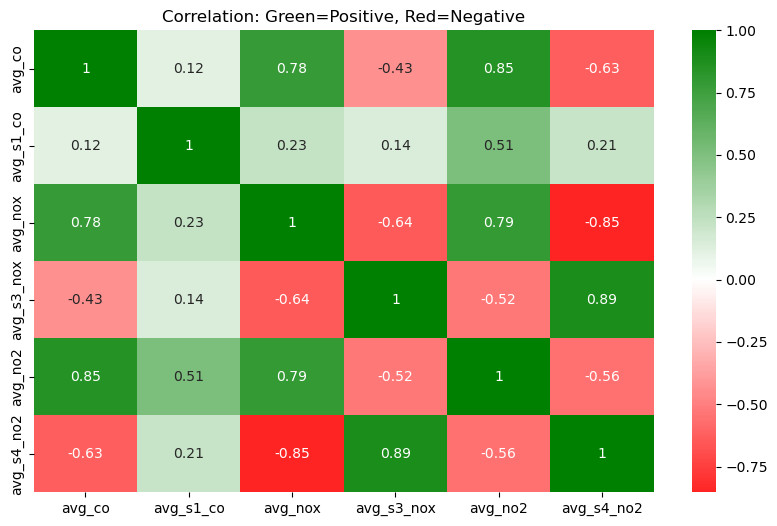
plt.title("Correlation: Green=Positive, Red=Negative")
plt.show()

Insight(s): There are strong positive correlations for the below -
- avg_co vs. avg_no2 ≈ 0.85
- avg_co vs. avg_nox ≈ 0.78
- avg_s3_nox vs. avg_s4_no2 ≈ 0.89
CO levels are surprisingly well correlated with NO₂ and NOₓ. This suggests that in the environment where the data was collected, these pollutants tend to rise and fall together. This could likely be due to common sources such as traffic. The S3 and S4 sensors, which measure NOX and NO2, appear to exhibit high cross-sensitivity to Ozone (O3). In other words, the high correlation between PT08.S3 (NOx) and PT08.S4 (NO₂) suggests that both are being influenced not just by NO or NO₂, but possibly by O₃ as well.
Conclusion
Air quality monitoring involves sensors that continuously emit readings. Hence, there is a need for high speeds in terms of data ingestion and retrieval. With its container models, GridDB serves as an excellent backend database for managing such multi-dimensional data points. In this analysis, we not only visualized air quality sensor discrepancies and seasonal trends but also showcased how the GridDB Cloud CLI enables quick data access, querying, and integration with GridDB Cloud — all with minimal infrastructure overhead. GridDB offers an open-source, scalable, and developer-friendly ecosystem built for the data-driven future of air quality management.
If you have any questions about the blog, please create a Stack Overflow post here https://stackoverflow.com/questions/ask?tags=griddb .
Make sure that you use the “griddb” tag so our engineers can quickly reply to your questions.