
Sales forecasting is processing of estimating future sales for a given period based on past data. Forecasting is a valuable tool that dictates the profitability of many companies and is thus an important skill to learn. It helps guide planning and direction for the company. There are several methods out there like Autoregressive Integrated Moving Average (ARIMA), Seasonal Autoregressive Integrated Moving-Average (SARIMA), Vector several (VAR), and so on. In this post we will use Keras for implementing a Long Short-term Memory (LSTM) model. LSTMs are a class of neural networks that are robust to feedback loops.
One for the main problems with Recurrent Neural networks is that over time, the information maintained in the hidden state gets overloaded. LSTMs maintain a additional hidden state that persists from step to step, this helps with the overloading. More details about LSTMs can be found here. We will use GridDB which is highly scalable and ensures high reliability, as a result it can serve as a great database for neural networks training and inference. Installing GridDB is simple and is well documented here. To check out the python-GridDB client please refer to this video.
LSTM
Setup
Let us setup GridDB first!
Quick setup of GridDB Python Client on Ubuntu 20.04:
- Install GridDB
Download and install the deb from here.
- Install C client
Download and install the Ubuntu from here.
- Install requirements
1) Swig console wget https://github.com/swig/swig/archive/refs/tags/v4.0.2.tar.gz tar xvfz v4.0.2.tar.gz cd swig-4.0.2 ./autogen.sh ./configure make
2) Install python client
wget
https://github.com/griddb/python_client/archive/refs/tags/0.8.4.zip
unzip . 0.8.4.zip
Make sure you have python-dev installed for the corresponding python version. We will use python 3.8 for this post.
3) We also need to point to the correct locations
export CPATH=$CPATH:<python header file directory path>
export LIBRARY_PATH=$LIBRARY_PATH:<c client library file directory path>
</c></python>
We can also use GridDB with docker as shown here
Python libraries
Next we install the python libraries. Installing plotly, numpy, keras, tensorflow and pandas is a simple pip install.
pip install keras
pip install numpy
pip install tensorflow
pip install plotly
pip install pandas
Prediction
Step 1: Downloading Dataset
we can download the data from this Kaggle project. The dataset contains Order Info, Sales, Customer, Shipping, etc., and can be used for Segmentation, customer analytics, clustering and so on. We will use it for sales forecasting, so we are only concerned with sales and order dates. We will predict monthly sales.
Step 2: Importing Libraries
import numpy as np
import pandas as pd
import plotly.offline as pyoff
import plotly.graph_objs as go
Step 3: Data Loading and Processing
Loading Data
data=pd.read_csv('/content/sales_data_sample.csv', encoding='cp1252') Note the encoding option used above.
Alternatively, we can use GridDB to get this data frame.
Feature Encoding
First, we collate the data at the monthly level. We simply se the date for each day to the first day of the month. Then we make average sales in the month. Note that not all days will have sales in each month.
data['ORDERDATE'] = pd.to_datetime(data['ORDERDATE'])
data['ORDERDATE'] = data['ORDERDATE'].dt.year.astype('str') + '-' + data['ORDERDATE'].dt.month.astype('str') + '-01'
data['ORDERDATE'] = pd.to_datetime(data['ORDERDATE'])
data = data.groupby('ORDERDATE').SALES.mean().reset_index()
Next, we plot the sales. We see some seasonality in the data, especially around the month of November.
plot_data = [
    go.Scatter(
        x=data['ORDERDATE'],
        y=data['SALES'],
    )
]
plot_layout = go.Layout(
        title='Monthly Sales'
    )
fig = go.Figure(data=plot_data, layout=plot_layout)
pyoff.iplot(fig) 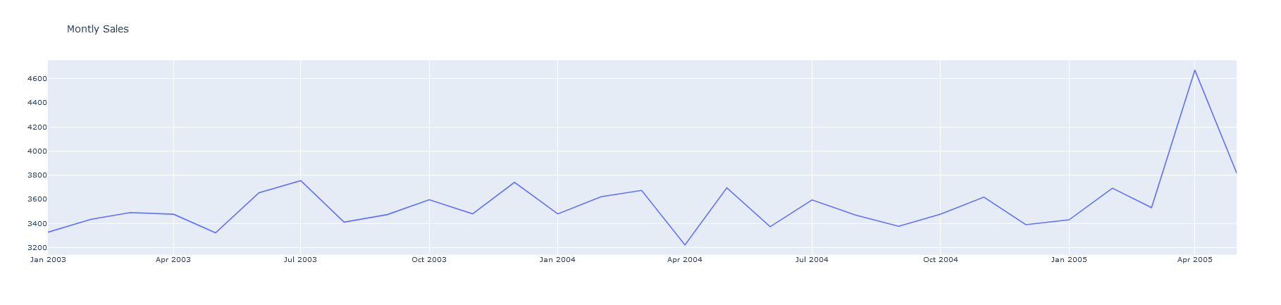
Next, we add a column for the difference of the sales, and drop the nulls, only the last values will be null as we cannot make a difference for that. The we create a few lags; lags allow the model to learn from not just the last but also the sales from before.
df_supervised = data.copy()
df_supervised['prev_sales'] = df_supervised['SALES'].shift(1)
df_supervised['diff'] = (df_supervised['SALES'] - df_supervised['prev_sales'])
df_supervised = df_supervised.drop(['prev_sales'],axis=1)
for inc in range(1,3):
    field_name = 'lag_' + str(inc)
    df_supervised[field_name] = df_supervised['diff'].shift(inc)
#drop null values
df_supervised = df_supervised.dropna().reset_index(drop=True)
Splitting Data into Validation and Train
Next, we split the data into tests and train. We have used the last 6 months to test.
from sklearn.preprocessing import MinMaxScaler
df_model = df_supervised.drop(['SALES','ORDERDATE'],axis=1)
#split train and test set
train_set, test_set = df_model[0:-6].values, df_model[-6:].values
We will also scale the data. Note that we scale the test and the train set separately. This is done so that the train and test sets remain independent.
#apply Min Max Scaler
scaler = MinMaxScaler(feature_range=(-1, 1))
scaler = scaler.fit(train_set)
# reshape training set
train_set = train_set.reshape(train_set.shape[0], train_set.shape[1])
train_set_scaled = scaler.transform(train_set)
# reshape test set
test_set = test_set.reshape(test_set.shape[0], test_set.shape[1])
test_set_scaled = scaler.transform(test_set)
X_train, y_train = train_set_scaled[:, 1:], train_set_scaled[:, 0:1]
X_train = X_train.reshape(X_train.shape[0], 1, X_train.shape[1])
X_test, y_test = test_set_scaled[:, 1:], test_set_scaled[:, 0:1]
X_test = X_test.reshape(X_test.shape[0], 1, X_test.shape[1]) Step 4: Prediction
Next, we start the prediction process.
Initializing
We first create an LSTM model in Keras. for that we use the LSTM layer.
# define the keras model
from keras.models import Sequential
from keras.layers import LSTM, Dense
model = Sequential()
model.add(LSTM(4, batch_input_shape=(1, X_train.shape[1], X_train.shape[2]), stateful=True))
model.add(Dense(1))
Training
Next, we compile the model. We use the mean_squared_error as the loss and evaluate it on accuracy.
model.compile(loss='mean_squared_error', optimizer='adam', metrics=['accuracy']) Next, we train the model for 100 epochs.
history=model.fit(X_train, y_train, epochs=100, batch_size=1, verbose=1, shuffle=False) Epoch 72/100
20/20 [==============================] - 0s 2ms/step - loss: 0.1302 - accuracy: 0.0000e+00
Epoch 73/100
20/20 [==============================] - 0s 2ms/step - loss: 0.1287 - accuracy: 0.0000e+00
Epoch 74/100
20/20 [==============================] - 0s 2ms/step - loss: 0.1272 - accuracy: 0.0000e+00
Epoch 75/100
20/20 [==============================] - 0s 2ms/step - loss: 0.1258 - accuracy: 0.0000e+00
Epoch 76/100
20/20 [==============================] - 0s 2ms/step - loss: 0.1244 - accuracy: 0.0000e+00 Evaluation and Predictions
Finally, we evaluate the test set, then we rescale the predictions and plot it along with the ground truth.
y_pred = model.predict(X_test,batch_size=1)
y_pred = y_pred.reshape(y_pred.shape[0], 1, y_pred.shape[1])

pred_test_set = []
for index in range(0,len(y_pred)):
    pred_test_set.append(np.concatenate([y_pred[index],X_test[index]],axis=1))

pred_test_set = np.array(pred_test_set)
pred_test_set = pred_test_set.reshape(pred_test_set.shape[0], pred_test_set.shape[2])
pred_test_set_inverted = scaler.inverse_transform(pred_test_set)

result_list = []
sales_dates = list(data[-7:].ORDERDATE)
act_sales = list(data[-7:].SALES)
for index in range(0,len(pred_test_set_inverted)):
    result_dict = {}
    result_dict['pred_value'] = int(pred_test_set_inverted[index][0] + act_sales[index])
    result_dict['ORDERDATE'] = sales_dates[index]
    result_list.append(result_dict)

df_result = pd.DataFrame(result_list)
#merge with actual sales dataframe
df_sales_pred = pd.merge(data,df_result,on='ORDERDATE',how='left')
#plot actual and predicted
plot_data = [
go.Scatter(
x=df_sales_pred['ORDERDATE'],
y=df_sales_pred['SALES'],
name='actual'
),
go.Scatter(
x=df_sales_pred['ORDERDATE'],
y=df_sales_pred['pred_value'],
name='predicted'
)
]
plot_layout = go.Layout(
title='Sales Prediction'
)
fig = go.Figure(data=plot_data, layout=plot_layout)
pyoff.iplot(fig) 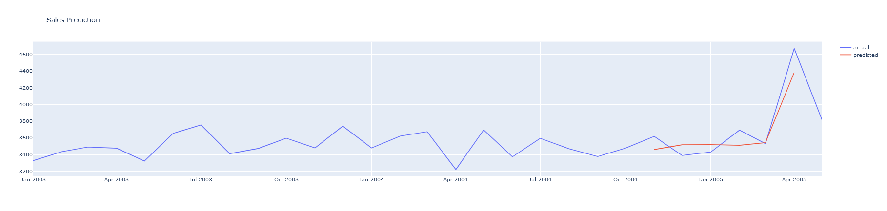
We see that the predictions are close. and off by a few 100. This shows the power of forecasting where we can get a close enough prediction in a matter of minutes with a quite simple model.
Conclusion
In this post we learned how to train an LSTM forecasting model with Keras, python and gridDB.