Step-By-Step Guide to Collecting & Visualizing Historical Cryptocurrency Market Data with GridDB

This blog is a continuation of our previous cryptocurrency blog found here

With Bitcoin currently leading the cryptocurrency market, as of this writing, its market cap stands at $1,083,949,725,691l; and by the time we publish this blog post, it may go even higher, all thanks to its high volatility.

Satoshi Nakamoto invented the Bitcoin network in 2009, which was then followed by the cryptocurrency’s first-ever recorded commercial transaction where Laszlo Hanyecz, a programmer, purchased two Papa John’s Pizza for 10,000 bitcoins. Back then, the coin didn’t hold any real value and wasn’t that big of a deal. But in the past decade, we have witnessed a massive surge, as the coin keeps crossing all-time highs. As of this writing, Bitcoin’s current value stands at $55,000+ per coin.

If the word of a few of the experts is to be believed, the coin will cross the $100,000 mark soon.Similarly, cryptocurrencies like Ethereum, Binance Coin, XRP, ADA, and various others have been predicted to skyrocket in the next few years. Their prices have been predicted to surge at an exponential rate as well.

The ever-increasing prices of different cryptocurrencies have been attracting countless retail as well as institutional investors from all across the world. Unlike the traditional financial markets, the cryptocurrency market is highly volatile and unpredictable. While financial markets are predictable, the same isn’t the case with the cryptocurrency market, thanks to its decentralized way of working, growing interest, and high volatility.

That’s the reason investors and traders all across the world have been looking for fast and reliable analysis tools to stay ahead in the game, helping them make bold predictions in this ever-growing dynamic market. So, to help them with their goals in a much efficient manner, we’ve come up with a fairly easy way of collecting historical cryptocurrency market data with the help of GridDB, which we’ll later visualize using Python.

This blog post focuses on collecting historical cryptocurrency market data from the Coingecko API and storing it in a GridDB, and further visualizing it using a Python script. Before we dive in, let’s look at the technologies we’ll be using:

The Technologies We’ll Be Using to Achieve Our Goal

Following are the technologies we’ll be building our tool on top of:

• OS: Ubuntu 18.04
• Python 3.6
• GridDB c Client: v4.5.0
• GridDB Server: latest version
• GridDB Python Client: 0.8.3

Fetching & Visualizing the Data

Day-to-day cryptocurrency market data can be fetched via numerous tactics. However, right now, our focus will be on collecting and visualizing the historical data of both Bitcoin and Ethereum.

First, let’s do it for Bitcoin. While Bitcoin was officially created in 2009, you won’t be able to fetch the data for the first few years, as the coin wasn’t traded publicly. Obviously, there exist transactions in the first blocks of the chain; however, back then, the price wasn’t controlled by the market.

Now, we’ll be fetching its historical data from the Coingecko API. To do that, we need to install the Python client using the command:

python3.6 -m pip install pycoingecko

We’re now about to write the Python script, which will help us collect and visualize the historical Bitcoin and Ethereum market data from the Coingecko API.

Let’s start writing our python script.

Step I: We’ll import the CoinGecko API.

from pycoingecko import CoinGeckoAPI

Step II: Now, we will import Matplotlib (for data visualization), Pandas, Numpy and Scipy.

install matplotlib.pylot as plt
import pandas as pd
import numpy as np
import scipy as sp

Step III: Here, we are creating the Coingecko APIs instance:

coingecko = CoinGeckoAPI()

Step IV: Next, we will define the functions to be used. We’ll get our hands on a given cryptocurrency’s market data with the get_coin_by_id() API call. The data fetched will be saved in the cryptocurrency_data.csv.

def get_data(cryptocurrency):
    cryptocurrency_data = coingecko.get_coin_by_id(cryptocurrency, market_data='true', sparkline='true')
    df = pd.DataFrame.from_dict(cryptocurrency_data, orient='index')
    df.to_csv(r'cryptocurrency_data.csv')
    return df

Step V: Let’s fetch the data for both Bitcoin and Ethereum.

get_data('bitcoin')

get_data('ethereum')

Now, you can see two cryptocurrency_data.csv files. Let’s open them one by one.

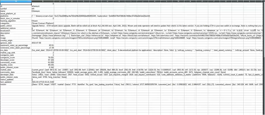
Here’s what Bitcoin’s CSV file looks like:

And the next CSV represents Ethereum’s market data:

Step VI: Our end-game is to get our hands on the Bitcoin and Ethereum historical market data and ultimately visualize it, so we’ll now define a function get_historical_data() to serve the purpose.

According to the official documentation, the data presented depends on the number of days. If we are tracking one-day Bitcoin data, then it’ll be presented in minutes. However, if we track historical data ranging from 2-90 days, then the data will be divided and presented in hours.

For more than 90 days, it’ll be divided and presented on a daily basis.

def get_historical_data(cryptocurrency, fiat_currency, number_of_days):
    historic_price = coingecko.get_coin_market_chart_by_id(cryptocurrency, fiat_currency, number_of_days)
    prices = [price[1] for price in historic_price['prices']]
    return prices

Here, the variable “prices” is a list.

For example, for the function:

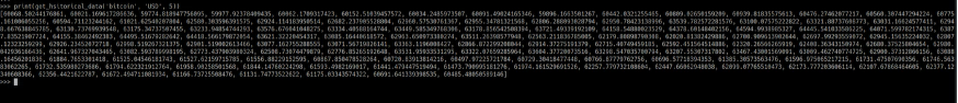
    print(get_historical_data('bitcoin', 'USD', 5))

The output will be:

Let’s further divide this post into two sections, where Section I represents collecting and visualizing 30-days Ethereum data, and Section II represents the same for Bitcoin.

Section I: Collecting & Visualizing the Past 30-Days Ethereum Market Data

Step I: Let’s capture the past 30 days data for Ethereum and store it in a variable like we did for Bitcoin

    ethereum = get_historical_data('ethereum', 'USD', 30)

Step II: Let’s save this data in Ethereum.csv.

    et_df = pd.DataFrame(ethereum, columns = ['Ethereum Value'])
    et_df.index.name = 'Every Hour Count in the Past 30 Days'
    et_df.to_csv(r'Ethereum.csv')
    df = pd.read_csv("Ethereum.csv")

Here, we are storing all of the generated data in Ethereum.csv. Now, let’s load it into the GridDB database.

Step III: Now, we’ll be initializing the GridDB database parameters.

    factory = griddb.StoreFactory.get_instance()
    argv = sys.argv
    try:
    #Get GridStore object
    gridstore = factory.get_store(
        notification_member="griddb-server:10001",
        cluster_name="defaultCluster",
        username="admin",
        password="admin"
    )

Step IV: Now, we will create a data frame for our CSV file.

    ethereum_data = pd.read_csv("/ethereum.csv", na_values=['\\N'])
    ethereum_data.info()

Here’s what we’ll get:

Step V: Now, let’s interact with the database. The usual way of interacting with the GridDB container is to create a container in it and load the information using the put or multi_put function.

So, let’s create the container ethereum_container for storing the data. Now, here the most important point to keep in mind is to make sure that the correct data types are defined, otherwise it may cause errors while performing the database operations.

    ethereum_container = "ETHEREUM"
    ethereum_containerInfo = griddb.ContainerInfo(ethereum_container,
    [["count", griddb.Type.INTEGER],["value", griddb.Type.STRING]],
    griddb.ContainerType.COLLECTION, True)
    ethereum_columns = gridstore.put_container(ethereum_containerInfo)
    ethereum_columns.create_index("count", griddb.IndexType.DEFAULT)
    ethereum_columns.put_rows(ethereum_data)    
    print("Data added successfully")    
    db_data = gridstore.get_container(ethereum_container)

Once we have created the container, we loaded the data using the put_rows function. When loaded, the “Data added successfully” message will appear in front of you.

Step VI: Now, let’s play around a bit and run some queries.

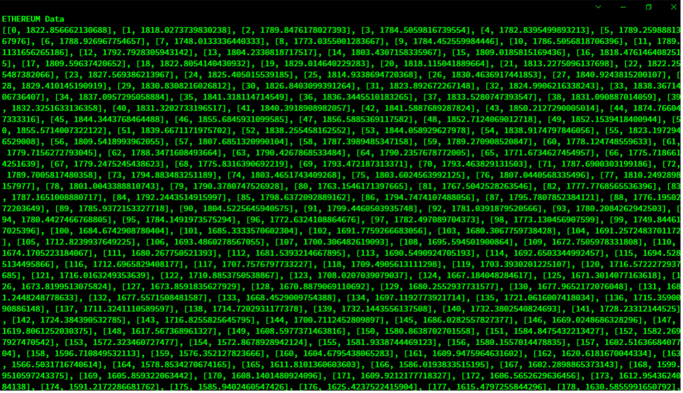
Query 1: First of all, let’s fetch all of that Ethereum data we loaded using the “Select *” query.

    query = db_data.query("Select *")
    rs = query.fetch(False)
    print(f"{ethereum_container} Data")
    retrieved_data = []
    while rs.has_next():
        data = rs.next()
        retrieved_data = append(newdata)
        print(retrieved_data)

Output:

Query 2: Let’s fetch Ethereum’s value for the seventh hour on Day I of the 30 days data we are tracking.

    query = db_data.query("select * where count = 7")
    rs = query.fetch(False)
    print(f"{ethereum_container} Data")
    retrieved_data = []
    while rs.has_next():
        data = rs.next()
        retrieved_data = append(newdata)
        print(retrieved_data)

Output:

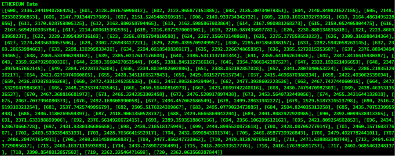
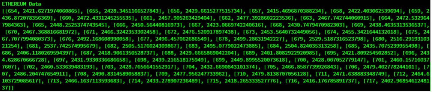
Query 3: Let’s fetch some recent data.

    query = db_data.query("select * where count >= 600")
    rs = query.fetch(False)
    print(f"{ethereum_container} Data")
    retrieved_data = []
    while rs.has_next():
        data = rs.next()
        retrieved_data = append(newdata)
        print(retrieved_data)

Output:

Query 4: Let’s fetch the time period when the Ethereum value crossed $2,400.

    query = db_data.query("select * where value > 2400")
    rs = query.fetch(False)
    print(f"{ethereum_container} Data")
    retrieved_data = []
    while rs.has_next():
        data = rs.next()
        retrieved_data = append(newdata)
        print(retrieved_data)

Output:

Query V: Let’s do the same for values above $2,000.

    query = db_data.query("select * where value >2000")
    rs = query.fetch(False)
    print(f"{ethereum_container} Data")
    retrieved_data = []
    while rs.has_next():
        data = rs.next()
        retrieved_data = append(newdata)
        print(retrieved_data)

Output:

Step VII: We’ll use this piece of code to avoid any exceptions.

    except griddb.GSException as e:
    for i in range(e.get_error_stack_size()):
        print("[", i, "]")
        print(e.get_error_code(i))
        print(e.get_location(i))
        print(e.get_message(i))

Step VIII: Finally, it’s time to visualize the data.

1. Scatter Plot:

    df.plot(x = 'Every Hour Count in the Past 30 Days', y = 'Ethereum Value', kind = 'scatter')
    plt.xlabel('Every Hour Count in the Past 30 Days')
    plt.ylabel('Ethereum Value')
    plt.show()

Graph:

1. Line Graph:

    df.plot(x = 'Every Hour Count in the Past 30 Days', y = 'Ethereum Value', kind = 'line')
    plt.xlabel('Every Hour Count in the Past 30 Days')
    plt.ylabel('Ethereum Value')
    plt.show()

Graph:

1. Bar:

    df.plot(x = 'Every Hour Count in the Past 30 Days', y = 'Ethereum Value', kind = 'bar')
    plt.xlabel('Every Hour Count in the Past 30 Days')
    plt.ylabel('Ethereum Value')
    plt.show()

Graph:

1. Autocorrelogram or Autocorrelation Plot using Statsmodel:

    import statsmodel.api as sm
    sm.graphics.tsa.plot_acf(df["Ethereum Value"])
    plt.show()

Graph:

Now that we have visualized the Ethereum market data from the past 30 days let’s do the same for Bitcoin.

Section I: Collecting & Visualizing the Past 30-Days Bitcoin Market Data

Step I: Let’s fetch the Bitcoin’s data from the past 30 days and store this list in a variable for better analysis.

    bitcoin = get_historical_data('bitcoin', 'USD', 30)

Step II: Now, we will save all of this data in a CSV.

    bt_df = pd.DataFrame(bitcoin, columns = ['Bitcoin Value'])
    bt_df.index.name = 'Every Hour Count in the Past 30 Days'
    bt_df.to_csv(r'Bitcoin.csv')
    df = pd.read_csv("Bitcoin.csv")

Here, we are storing all of the generated data in Bitcoin.csv. We can also load all of Bitcoin’s data into the GridDB database, but here we will just be visualizing it.

Step III: Let’s visualize it.

1. Scatter Plot:

    df.plot(x = 'Every Hour Count in the Past 30 Days', y = 'Bitcoin Value', kind = 'scatter')
    plt.xlabel('Every Hour Count in the Past 30 Days')
    plt.ylabel('Bitcoin Value')
    plt.show()

Graph:

1. Line Graph:

    df.plot(x = 'Every Hour Count in the Past 30 Days', y = 'Bitcoin Value', kind = 'line')
    plt.xlabel('Every Hour Count in the Past 30 Days')
    plt.ylabel('Bitcoin Value')
    plt.show()

Graph:

1. Bar:

    df.plot(x = 'Every Hour Count in the Past 30 Days', y = 'Bitcoin Value', kind = 'bar')
    plt.xlabel('Every Hour Count in the Past 30 Days')
    plt.ylabel('Bitcoin Value')
    plt.show()

Graph:

Note: We are tracking every single hour’s data for the past 30 days, which is why all the values in the X-Axis are colliding.

Autocorrelogram or Autocorrelation Plot using Statsmodel:

    import statsmodel.api as sm
    sm.graphics.tsa.plot_acf(df["Bitcoin Value"])
    plt.show()

Graph:

Similarly, we can capture and visualize historical data of other cryptocurrencies supported by Coingecko API.

Conclusion

If you have been planning to invest in Bitcoin, Ethereum, or other cryptocurrencies, you can conduct your research by collecting and visualizing data as we did in this blog post.

The full source code can be found here: GitHub

If you have any questions about the blog, please create a Stack Overflow post here https://stackoverflow.com/questions/ask?tags=griddb .
Make sure that you use the “griddb” tag so our engineers can quickly reply to your questions.