Time Series Classification with Amazon Chronos Model with GridDB

This article shows how to build a time series forecasting model for electricity production using Amazon Chronos and GridDB database.

We will retrieve historical electricity production data from Kaggle, insert it into a GridDB time series container, and use the data to train a forecasting model with Amazon Chronos, a specialized collection of time series models based on the T5 architecture.

GridDB is a robust NOSQL database optimized for efficiently handling large volumes of real-time data. Its advanced in-memory processing and time series data management make it ideal for big data and IoT applications.

GridDB’s real-time data processing capabilities and Chronos’ state-of-the-art forecasting methods make them a powerful combination for time forecasting applications.

Prerequisites

You need to install the following libraries to run codes in this article.

1. GridDB C Client
2. GridDB Python client

Instructions for installing these clients are available on GridDB Python Package Index (Pypi).

You must also install Amazon Chronos, Numpy, Pandas, and Matplotlib libraries.

The scripts below will help you install and import the necessary libraries for running codes.

%pip install git+https://github.com/amazon-science/chronos-forecasting.git
%pip install matplotlib seaborn numpy pandas scikit-learn

import matplotlib.pyplot as plt
from matplotlib.dates import DateFormatter
import seaborn as sns
import numpy as np
import pandas as pd
import torch
from chronos import ChronosPipeline
import griddb_python as griddb
from sklearn.metrics import mean_absolute_error

Inserting Time Series Data Into GriddB

The first step is to insert the time series data we want to forecast into GridDB. This section explains the steps involved.

Downloading and Importing Electricity Production Data from Kaggle

We will forecast future electricity production requirements using the Electricity Production dataset from Kaggle.

The following script imports the CSV file containing the dataset into a pandas DataFrame.

dataset = pd.read_csv("Electric_Production.csv")
dataset.head(10)

Output:

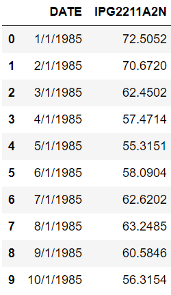
The dataset consists of monthly electricity production from 1st January 1985 to 1st January 2018.

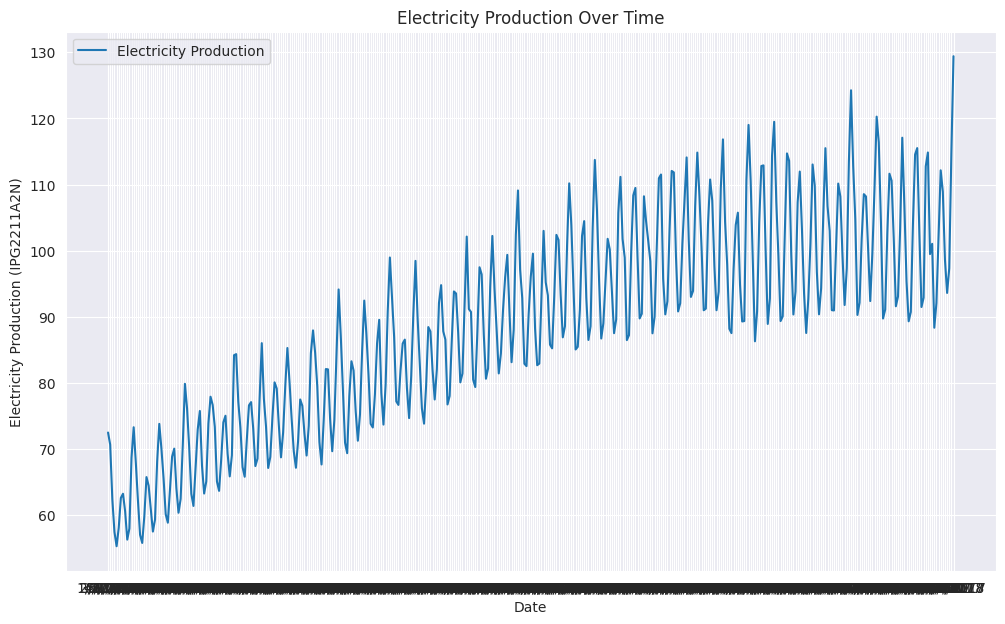
You can draw line plots to see that electricity production highly depends on the month of the year.

# Create the line plot
sns.set_style("darkgrid")
plt.figure(figsize=(12, 7))
sns.lineplot(data=dataset, x='DATE', y='IPG2211A2N', label='Electricity Production')
plt.xlabel('Date')
plt.ylabel('Electricity Production (IPG2211A2N)')
plt.title('Electricity Production Over Time')
plt.legend()

plt.show()

Output:

Once we have our dataset, we can insert this data into GridDB.

Connect to GriddB

To connect to GridDB, you need to create an object of the StoreFactory class. Next, call the get_store() method on the store factory object and pass the DB host and cluster names, user, and password.

To test if the connection is successful, call the get_container() method and pass it the name of any container. If you see the following output, your connection is successful.

# GridDB connection details
DB_HOST = "127.0.0.1:10001"
DB_CLUSTER = "myCluster"
DB_USER = "admin"
DB_PASS = "admin"

# creating a connection

factory = griddb.StoreFactory.get_instance()

try:
    gridstore = factory.get_store(
        notification_member = DB_HOST,
        cluster_name = DB_CLUSTER,
        username = DB_USER,
        password = DB_PASS
    )

    container1 = gridstore.get_container("container1")
    if container1 == None:
        print("Container does not exist")
    print("Successfully connected to GridDB")

except griddb.GSException as e:
    for i in range(e.get_error_stack_size()):
        print("[", i, "]")
        print(e.get_error_code(i))
        print(e.get_location(i))
        print(e.get_message(i))

Output:

Container does not exist
Successfully connected to GridDB

Create Container for Electricity Production Data in GridDB

GrirDB stores data containers. You need the container name and column information to create a container.

You can assign any name to your container. However, the container information must be a list of lists, each nested list containing the column name and the column type.

For example, in the script below we have two columns: TimeStamp with column type griddb.Type.TIMESTAP, and Production with griddb.Type.DOUBLE type.

Next, you need to create an object of the ContainerInfo class and pass the container name and column info to the ContainerInfo class constructor.

Finally, call the put_container() method and pass to it the ContainerInfo class object to create a container in the GridDB.

dataset['DATE'] = pd.to_datetime(dataset['DATE'])


container_name = "Electricity_Production"
column_info = [
    ["Timestamp", griddb.Type.TIMESTAMP],
    ["Production", griddb.Type.DOUBLE]
]
container_info = griddb.ContainerInfo(container_name, column_info, griddb.ContainerType.TIME_SERIES)

# Creating Container
try:
    gridstore.put_container(container_info)
    container = gridstore.get_container(container_name)
    if container is None:
        print(f"Failed to create container: {container_name}")
    else:
        print(f"Successfully created container: {container_name}")

except griddb.GSException as e:
    print(f"Error creating or retrieving container {container_name}:")
    for i in range(e.get_error_stack_size()):
        print(f"[{i}]")
        print(f"Error code: {e.get_error_code(i)}")
        print(f"Location: {e.get_location(i)}")
        print(f"Message: {e.get_message(i)}")

Output

Successfully created container: Electricity_Production

You can retrieve the container you created using the get_container() method.

The next step is to store our dataset in the container we just created.

Insert Electricity Production Data into GridDB Container

To insert data into our GridDB container, we will iterate through all the rows in our dataset, call our container object’s put() method, and pass the values from the DATE and IPG2211A2N columns to the method.

try:
    for index, row in dataset.iterrows():
        container.put([row['DATE'].to_pydatetime(), row['IPG2211A2N']])
    print(f"Successfully inserted {len(dataset)} rows of data into {container_name}")

except griddb.GSException as e:
    print(f"Error inserting data into container {container_name}:")
    for i in range(e.get_error_stack_size()):
        print(f"[{i}]")
        print(f"Error code: {e.get_error_code(i)}")
        print(f"Location: {e.get_location(i)}")
        print(f"Message: {e.get_message(i)}")

Output

Successfully inserted 397 rows of data into Electricity_Production

We have successfully inserted the electricity production data into the GridDB. The next step is to forecast electricity production using Amazon’s Chronos model.

Forecasting Electricity Production using Amazon’s Chronos Time Series Model

Amazon Chronos is a collection of pre-trained language models specifically designed for time series forecasting. These models are based on the T5 (Text-to-Text Transfer Transformer) architecture, which has been adapted to handle time series data.

Retrieving Data from GridDB

We first need to retrieve data we stored in GridDB to forecast electricity production. To do so, you can use the get_container() method and pass it the container name you want to retrieve.

Call the SELECT * query using the container’s query() method. Next, call the fetch() method to retrieve the dataset object. Finally, call the fetch_rows() method to store the dataset into a pandas DataFrame.

def retrieve_data_from_griddb(container_name):

    try:
        stock_data_container = gridstore.get_container(container_name)

        # Query all data from the container
        query = stock_data_container.query("select *")
        rs = query.fetch()  # Adjust the number based on your data size

        data = rs.fetch_rows()
        data .set_index("Timestamp", inplace=True)
        return data

    except griddb.GSException as e:
        print(f"Error retrieving data from GridDB: {e.get_message()}")
        return None


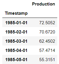
electric_production_data = retrieve_data_from_griddb("Electricity_Production")
electric_production_data.head()

Output:

Forecasting Electricity Production using Amazon Chronos Model

Amazon Chronos models are available for free on Hugging Face. For making inferences, you can simply install the model from GitHub.

We will divide our dataset into a training and test set. Then, we will use the Amazon Chronos model to forecast electricity production for the months in the test set. Finally, we will evaluate the model’s performance by comparing the forecasted electricity production with the actual production.

The following script divides the dataset into train and test sets. The dataset has a total of 397 records. We will use the last 47 records for testing.

# Define the test size and calculate the split index
test_size = 47
split_index = len(electric_production_data) - test_size

# Check if the data length is shorter than the test size
if split_index < 0:
    train_production = pd.Series(dtype=float)
    test_production = electric_production_data['Production']
else:
    # Splitting the Production column into training and test sets
    train_production = electric_production_data['Production'].iloc[:split_index]
    test_production = electric_production_data['Production'].iloc[split_index:]

# Display the results
print("Training Set:")
print(train_production.shape)
print("\nTest Set:")
print(test_production.shape)

Output:

Training Set:
(350,)

Test Set:
(47,)

Next, we will import the pretrained Chronos t5 large model using the ChronosPipeline.from_pretrained() method.

pipeline = ChronosPipeline.from_pretrained(
  "amazon/chronos-t5-large",
  device_map="cuda",
  torch_dtype=torch.bfloat16,
)

Chronos models expect data to be in torch tensor format. The script below converts the data into torch tensors. Next, we use the pipeline.predict() method to forecast the next 47 months of electricity production based on the training data (context).

We divide the predictions into three quantiles (0.1, 0.5, 0.9).

context = torch.tensor(train_production)
prediction_length = test_size
forecast = pipeline.predict(context, prediction_length)
low, median, high = np.quantile(forecast[0].numpy(), [0.1, 0.5, 0.9], axis=0)

Next, we evaluate the model performance.

Evaluating Model Performance

We will plot the median forecast values against the test values. To do so, we will create a pandas DataFrame that contains our predictions.

The following script plots the training set, test set, and predictions.

test_production.index = pd.to_datetime(test_production.index)
median_forecast = pd.Series(median, index=test_production.index, name="Median Forecast")

plt.figure(figsize=(12, 6))
plt.plot(train_production.index, train_production, color='blue', label="Training Set", linestyle="-")
plt.plot(test_production.index, test_production, color='green', linestyle="--", label="Test Set")
plt.plot(median_forecast.index, median_forecast, color='red', linestyle=":", label="Median Forecast")

# Vertical line to mark the start of the test set
plt.axvline(x=test_production.index[0], color='black', linestyle="--", label="Test Set Start")

plt.xlabel("Timestamp")
plt.ylabel("Production")
plt.title("Production - Training, Test, and Predictions (Median Forecast)")
plt.legend()
plt.show() 

Output:

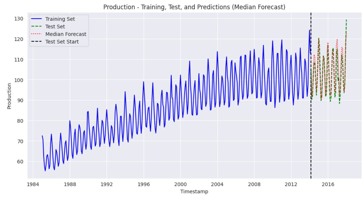
The above output shows that our model performs well and can capture the trends in the training dataset. The predictions are close to the values in the test set.

Next, we will plot only the test values against the median prediction values and the 80% prediction interval.

median_forecast = pd.Series(median, index=test_production.index, name="Median Forecast")
lower_bound = pd.Series(low, index=test_production.index, name="Lower Bound")
upper_bound = pd.Series(high, index=test_production.index, name="Upper Bound")


plt.figure(figsize=(12, 6))

plt.plot(test_production.index, test_production, color='green', linestyle=":", label="Actual Production")
plt.plot(median_forecast.index, median_forecast, color='red', linestyle=":", label="Median Forecast")

# Plot the 80% prediction interval as an orange shaded area
plt.fill_between(test_production.index, lower_bound, upper_bound, color='orange', alpha=0.3, label="80% Prediction Interval")

plt.xlabel("Timestamp")
plt.ylabel("Production")
plt.title("Production - Actual vs. Forecast with 80% Prediction Interval")
plt.legend()
plt.show()

Output:

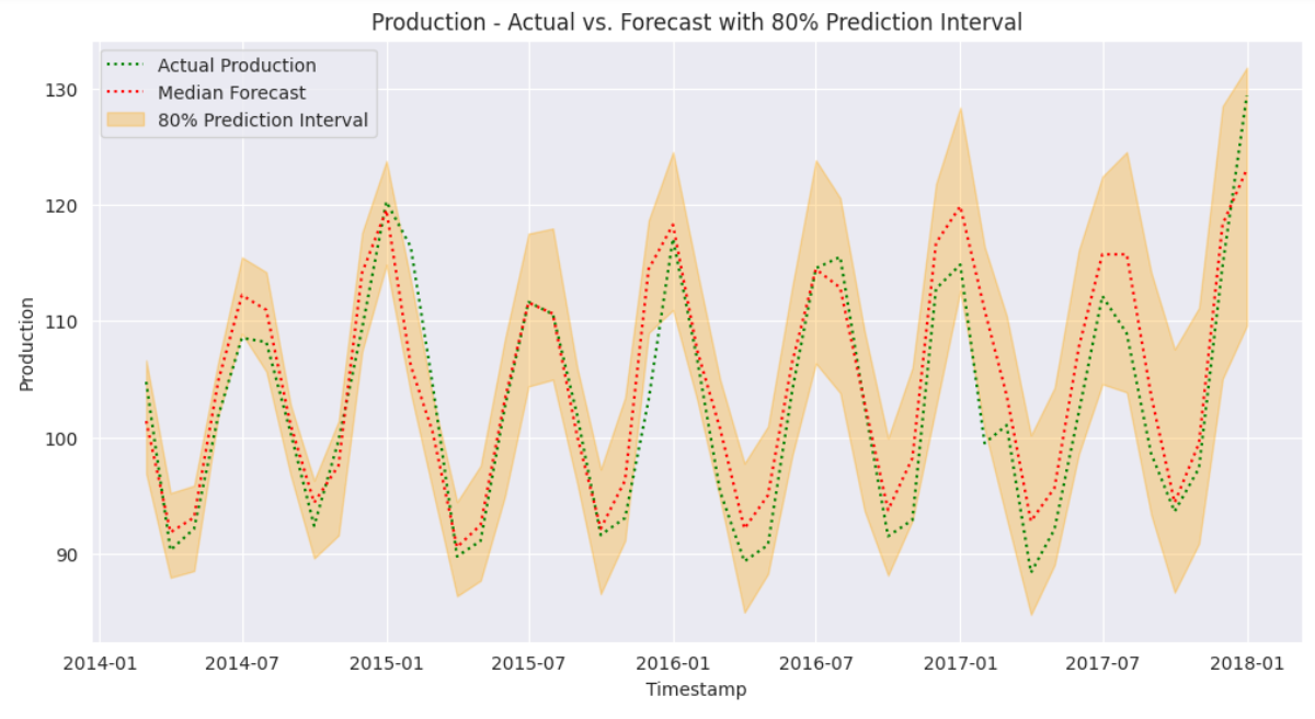
The above output shows that prediction values in 80% intervals cover almost all the test data, showing that our model performs exceptionally well for forecasting time series data.

Finally, we will plot the mean absolute error (MAE) values for the predictions to quantify the results.

mae = mean_absolute_error(test_production, median_forecast)

# Print results
print("Average electricity production values in the training set:", train_production.mean())
print("Mean Absolute Error (MAE):", mae)

Output:

Average electricity production values in the training set: 86.9775362857143
Mean Absolute Error (MAE): 3.2303302385930803

We obtain an MAE value of 3.23, indicating that, on average, our model’s predictions are only 3.23 units off from the actual test values, just a 3.4% deviation from the average electricity production in the training set.

Conclusion

This article covered the complete workflow for time series forecasting with GridDB and Amazon Chronos. You saw how to connect to GridDB, insert time series data, and train an Amazon Chronos model to forecast electricity production. The results showed accurate predictions, capturing seasonal trends and providing reliable forecasts within an 80% confidence interval.

Combining GridDB’s robust time series data management with Chronos’ specialized forecasting models provides a scalable solution for accurate time-series predictions.

If you have any questions about the blog, please create a Stack Overflow post here https://stackoverflow.com/questions/ask?tags=griddb .
Make sure that you use the “griddb” tag so our engineers can quickly reply to your questions.