ある人(完全なオタクか、大規模なカスタムPC構築会社)が、自分たちが構築したゲーミングPCの性能を記録したいと考えたとします。同社の場合、同じコンポーネントを搭載したシステム間の性能を統一することで、故障したシステムの出荷を回避することができるのです。オタクの場合は、非問題の解決策を大量に作りすぎたという自負が湧いてくるのでしょう。
CapFrameX は、Microsoft Windows用のオープンソースソフトウェアで、ゲームのパフォーマンス、FPS(Frame Per Second)やフレームタイム、CPU温度やグラフィックカードの消費電力などのコンポーネントセンサーデータを追跡することができます。CapFrameXは、ゲーム実行中にこれらのデータを表示することができますが、JSONファイルに保存することも可能です。
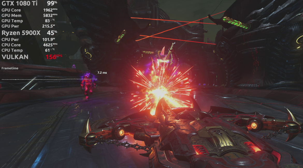
フレーム時間ごとにログを取ると、当然ながら膨大な量のデータが生成されます。スクリーンショットを見ると、現在のフレームはレンダリングに7.2msかかっています。つまり、1秒間に約150のデータポイントが生成されており、それをすべてログに取り込みたいのです。つまり、30分のゲームプレイデータを取得すると、約30万件のデータポイントになります。
最初のステップは、JSONファイルからデータを抽出し、GridDBデータベースの適切なテーブル構造にデータをロードすることです。
本記事のソースコード全文はこちらからご覧いただけます。 ソースコード
JSONからCapFrameXのデータを抽出する。
# The data and entire project is available for download at:
# https://github.com/retowyss/pc-benchmarking-r-griddb

library(tidyverse)
library(jsonlite)

# This is just some janitorial data wrangling
# The function reads the data captured by CapFrameX and makes it available
# in a easy to use format.
# Returns a list of three things: system-info, capture-data, sensor-data
read_capframex_json <- function(x) {
  capframe_data <- read_json(x, simplifyVector = TRUE)

  # We need a common length for the captured sensor data because some rows
  # are length n and some are n-k
  common_n <- length(capframe_data$Runs$SensorData2$MeasureTime$Values[[1]])

  list(
    info    = capframe_data$Info %>%
      keep(~!is.null(.)) %>%
      as_tibble(),
    capture = as_tibble(map(capframe_data$Runs$CaptureData, ~ .[[1]])),
    sensors = imap_dfc(capframe_data$Runs$SensorData2, function(df, names) {

      m <- length(df$Values[[1]])
      vals <- vector(mode = typeof(df$Values[[1]]), common_n)

      # if vector is shorter, we fill last value
      if(m < common_n) {
        vals <- c(df$Values[[1]], rep(df$Values[[1]][m], common_n - m))
      } else {
        vals <- (df$Value[[1]])[1:common_n]
      }

      res <- list()
      # Some list names are not appropriate as tibble headers
      n <- str_remove(str_replace_all(names, "/", "_"), "_")
      res[[n]] <- vals

      as_tibble(res)
    })
  )
}

capframex_data <- read_capframex_json("data/CapFrameX-DOOMEternalx64vk.exe-2.json")
私たちの目的のために、必要最小限のデータしか残しませんが、他にもたくさんありますので、自由に調べてみてください。
キャプチャデータは1フレームにつき1つのデータポイント(MsBetweenPresents)を作成するため、一定の時間ウィンドウでキャプチャした場合の行数は可変となります。ただし、センサーデータは250msという比較的一定の間隔(BetweenMeasureTime)でポーリングされていますが、多少のばらつきがあることが分かります。
capframex_data$info %>%
  select(Processor, GPU, SystemRam, GameName, OS, Motherboard) %>%
knitr::kable()| Processor | GPU | SystemRam | GameName | OS | Motherboard |
|---|---|---|---|---|---|
| AMD Ryzen 9 5900X | NVIDIA GeForce GTX 1080 Ti | 16GB (2x8GB) 3200MT/s | Doom Eternal | Microsoft Windows 11 Pro Build 22000 | Gigabyte Technology Co. Ltd. B550I AORUS PRO AX |
情報テーブルには、PCシステムのハードウェア(プロセッサー、GPU、RAM、マザーボード)およびソフトウェアデータ(ゲーム、オペレーティングシステム)が含まれています。
capframex_data$capture %>%
  select(TimeInSeconds, MsBetweenPresents) %>%
  head(n = 3) %>%
knitr::kable()| TimeInSeconds | MsBetweenPresents |
|---|---|
| 0.0000000 | 8.2026 |
| 0.0058994 | 5.8994 |
| 0.0142062 | 8.3068 |
キャプチャテーブルにはパフォーマンスデータが含まれています。time = 0 (TimeInSeconds) で記録された最初のフレームは、ハードウェアのレンダリングに 8.2ms (MsBetweenPresents) を要しました。2番目のフレームは5.9ms(MsBetweenPresents)かかったので、セッションの開始時点と比較して0.0059(TimeInSeconds)秒経過しています。
より良いハードウェアは、1フレームあたりの使用時間が短く、より多くのフレーム/秒(FPS)を生成するため、ゲーム内のアニメーションがより滑らかに見えることから、このパフォーマンスデータと呼んでいます。しかし、知覚される滑らかさは、ハードウェアがレンダリングできるフレーム数だけでなく、フレーム間の時間のばらつきにも影響されます(ばらつきは少ない方が良い)。その為、平均フレームタイムが良好(低い)であっても、フレームタイムに大きな突出が繰り返される場合は、性能上の問題があることを示す指標となり得ます。
TimeInSeconds: セッションが開始されてからの時間(秒)MsBetweenPresents: 現在のフレームのレンダリングにかかった時間。実質的にはTimeInSeconds(n) –TimeInSeconds(n – 1)
capframex_data$sensors %>%
  select(MeasureTime, BetweenMeasureTime,
   cpu_power = amdcpu_0_power_0,
   cpu_temperature = amdcpu_0_temperature_0,
   gpu_clock = nvidiagpu_0_clock_0,
   gpu_power = nvidiagpu_0_power_0,
   gpu_temperature = nvidiagpu_0_temperature_0
  ) %>%
  head(n = 2) %>%
knitr::kable()| MeasureTime | BetweenMeasureTime | cpu_power | cpu_temperature | gpu_clock | gpu_power | gpu_temperature |
|---|---|---|---|---|---|---|
| 0.004 | 0.004 | 106.7973 | 61.750 | 1961.5 | 234.502 | 80 |
| 0.265 | 0.261 | 108.1045 | 61.625 | 1961.5 | 211.884 | 80 |
センサーデータの MeasureTime は、キャプチャデータの TimeInSeconds と同じで、セッション開始からの時間を表しています。しかし、センサーデータは一定間隔でポーリングされ、新しいフレームが生成されたときではないため、データポイントは一対一に関連しません。
MeasureTime: セッションが開始されてからの時間(秒)BetweenMeasureTime: 前回測定時からの正確な時間(約250ms)cpu_power: CPU(プロセッサ)の消費電力(単位:ワット)cpu_temperature: CPUの温度(単位:℃)gpu_clock: GPU(グラフィックカード)のクロックスピード(MHz)gpu_power: GPUの消費電力(ワット)gpu_temperature: GPUの温度
CapFrameXのデータをGridDBに読み込む。
GridDBに3つのテーブル(Info、Capture、Sensor)を作成し、テーブルにjsonファイルを入力するための挿入関数を作成します。この過程で、リレーショナルデータ点を適切に参照するためのidを追加する必要があります。
# We are using a docker based setup that can run this project ootb
# it's available here: https://github.com/retowyss/rstudio-server-griddb-docker

# You can set this up without docker, the containers use:

# Latest version griddb                 https://docs.griddb.net
# Latest version of R and tidyverse     R >= 4.0.0
# Latest version of JDBC                https://github.com/griddb/jdbc

# For general setup without docker you can follow this post:
# https://griddb.net/en/blog/analyzing-nba-play-by-play-data-using-r-and-griddb/

library(RJDBC)
drv <- JDBC(
  driverClass = "com.toshiba.mwcloud.gs.sql.Driver",
  # Point this to your gridstore jar
  classPath = "/jdbc/bin/gridstore-jdbc.jar"
)

# IP and port depend on your setup
griddb <- dbConnect(
  drv,
  "jdbc:gs://172.20.0.42:20001/dockerGridDB/public",
  "admin",
  "admin"
)

# System info table: cfx_info
dbSendUpdate(griddb, paste(
  "CREATE TABLE IF NOT EXISTS cfx_info",
  "(id INTEGER, Processor STRING, GPU STRING, SystemRam STRING,",
  "GameName STRING, OS STRING, Motherboard STRING);"
))

# Frame time capture data: cfx_capture
dbSendUpdate(griddb, paste(
  "CREATE TABLE IF NOT EXISTS cfx_capture",
  "(info_id INTEGER, TimeInSeconds FLOAT, MsBetweenPresents FLOAT);"
))

# Sensor data: cfx_sensors
dbSendUpdate(griddb, paste(
  "CREATE TABLE IF NOT EXISTS cfx_sensors",
  "(info_id INTEGER, MeasureTime FLOAT, BetweenMeasureTime FLOAT,",
  "cpu_power FLOAT, cpu_temperature FLOAT, gpu_clock FLOAT, gpu_power FLOAT,",
  "gpu_temperature FLOAT);"
))

dbInsertTable <- function(conn, name, df, append = TRUE) {
  for (i in seq_len(nrow(df))) {
    dbWriteTable(conn, name, df[i, ], append = append)
  }
  invisible(TRUE)
}

# This is not a "production" ready approach of doing this, but it's sufficient
# for this demo :)
# Inserts dataset (cfx_data) into database (conn) using ID (uid)
insert_cfx_data <- function(conn, cfx_data, uid) {

  dbInsertTable(conn, "cfx_info",
    cfx_data$info %>%
      transmute(id = uid, Processor, GPU, SystemRam, GameName, OS, Motherboard)
  )

  dbInsertTable(conn, "cfx_capture",
    cfx_data$capture %>%
      transmute(info_id = uid, TimeInSeconds, MsBetweenPresents)
  )

  dbInsertTable(conn, "cfx_sensors",
    cfx_data$sensors %>%
      transmute(
        info_id = uid,
        MeasureTime,
        BetweenMeasureTime,
        cpu_power = amdcpu_0_power_0,
        cpu_temperature = amdcpu_0_temperature_0,
        gpu_clock = nvidiagpu_0_clock_0,
        gpu_power = nvidiagpu_0_power_0,
        gpu_temperature = nvidiagpu_0_temperature_0
      )
  )
  invisible(TRUE)
}
# Insert (this takes a while, don't run while knitting the doc)
json_files <- list.files("data")
walk2(json_files, 1:length(json_files), function(x, i) {
insert_cfx_data(griddb, read_capframex_json(paste0("data/", x)), i)
})単一のシステム(Ryzen 9 5900X、16GB RAM、Windows 11)を使ってデータを収集しましたが、複数のゲームをテストし、GTX 1650とGTX 1080 Tiという2種類のグラフィックカード(GPU)をテストしました。
# Check
dbGetQuery(griddb,"SELECT * FROM cfx_info;") %>%
knitr::kable()| id | Processor | GPU | SystemRam | GameName | OS | Motherboard |
|---|---|---|---|---|---|---|
| 1 | AMD Ryzen 9 5900X | NVIDIA GeForce GTX 1080 Ti | 16GB (2x8GB) 3200MT/s | Assassin’s Creed Valhalla | Microsoft Windows 11 Pro Build 22000 | Gigabyte Technology Co. Ltd. B550I AORUS PRO AX |
| 2 | AMD Ryzen 9 5900X | NVIDIA GeForce GTX 1650 | 16GB (2x8GB) 3200MT/s | Cyberpunk 2077 | Microsoft Windows 11 Pro Build 22000 | Gigabyte Technology Co. Ltd. B550I AORUS PRO AX |
| 3 | AMD Ryzen 9 5900X | NVIDIA GeForce GTX 1650 | 16GB (2x8GB) 3200MT/s | Doom Eternal | Microsoft Windows 11 Pro Build 22000 | Gigabyte Technology Co. Ltd. B550I AORUS PRO AX |
| 4 | AMD Ryzen 9 5900X | NVIDIA GeForce GTX 1080 Ti | 16GB (2x8GB) 3200MT/s | Doom Eternal | Microsoft Windows 11 Pro Build 22000 | Gigabyte Technology Co. Ltd. B550I AORUS PRO AX |
| 5 | AMD Ryzen 9 5900X | NVIDIA GeForce GTX 1650 | 16GB (2x8GB) 3200MT/s | ROLLERDROME | Microsoft Windows 11 Pro Build 22000 | Gigabyte Technology Co. Ltd. B550I AORUS PRO AX |
GridDBのデータベースには数ファイルしか入れていませんが、すでに約80万行のキャプチャデータがあります。
# Check
dbGetQuery(griddb,"SELECT COUNT(*) FROM cfx_capture;")
##
## 1 778780PCのパフォーマンスサマリーを作成する
私たちは今、特定のCPU、GPU、ゲームの組み合わせに対するパフォーマンスのサマリーを求めています。PCメーカーがこのアイデアを発展させ、同じハードウェアコンポーネントを使用した別のシステムとデータを比較することも可能です。 そうすることで、構築したシステムが期待通りの性能を発揮することを確認してから、お客様にお届けすることが出来るのです。
# We use paste and str_interp to build up our SQL in a readable and easy to
# understand way
get_performance_summary <- function(conn, cpu, gpu, game) {
  system_info <- paste(
    "SELECT ID",
    "FROM cfx_info",
    "WHERE Processor = '${cpu}' AND GPU = '${gpu}' AND GameName = '${game}'"
  )

  capture <- paste(
    "SELECT AVG(MsBetweenPresents) AS frame_time,",
    "MAX(TimeInSeconds) AS session_time,",
    "COUNT(*) AS frame_count",
    "FROM (", system_info, ") info",
    "LEFT JOIN (SELECT * FROM cfx_capture) capture",
    "ON info.id = capture.info_id"
  )

  sensors <- paste(
    "SELECT AVG(cpu_power) AS cpu_power, ",
    "AVG(cpu_temperature) AS cpu_temperature,",
    "AVG(gpu_clock) AS gpu_clock, AVG(gpu_power) AS gpu_power,",
    "AVG(gpu_temperature) AS gpu_temperature",
    "FROM (", system_info, ") info",
    "LEFT JOIN (SELECT * FROM cfx_sensors) sensors",
    "ON info.id = sensors.info_id"
  )

  capture_res <- dbGetQuery(conn, str_interp(capture))
  sensors_res <- dbGetQuery(conn, str_interp(sensors))

  as_tibble(bind_cols(
    tibble(cpu = cpu, gpu = gpu, game = game),
    capture_res %>%
      mutate(fps = 1000 / frame_time),
    sensors_res
  ))
}

gtx_1650_rollerdrome <- get_performance_summary(griddb,
  cpu =  "AMD Ryzen 9 5900X",
  gpu =  "NVIDIA GeForce GTX 1650",
  game = "ROLLERDROME"
)

glimpse(gtx_1650_rollerdrome)
## Rows: 1
## Columns: 12
## $ cpu <chr> "AMD Ryzen 9 5900X"
## $ gpu <chr> "NVIDIA GeForce GTX 1650"
## $ game <chr> "ROLLERDROME"
## $ frame_time <dbl> 2.660829
## $ session_time <dbl> 400.8515
## $ frame_count <dbl> 150650
## $ fps <dbl> 375.8227
## $ cpu_power <dbl> 95.65372
## $ cpu_temperature <dbl> 56.58357
## $ gpu_clock <dbl> 1848.533
## $ gpu_power <dbl> 74.72834
## $ gpu_temperature <dbl> 60.41905また、それをテキストパラグラフにして、システムレポートに記載することも出来ます。
summary2text <- function(summary_data) {
  spinable <- paste0(
    "Your system featuring a ${cpu} and ${gpu} performance in ",
    "a ${round(session_time/60)} minutes session of ${game} ",
    "was ${round(fps)} FPS.",
    "The graphics card used ${round(gpu_power)}W and ",
    "ran at ${round(gpu_temperature)}°C, ",
    "while the CPU used ${round(cpu_power)}W and ",
    "ran at ${round(cpu_temperature)}°C"
  )

  str_interp(spinable, env = summary_data)
}

summary2text(gtx_1650_rollerdrome)
## [1] "Your system featuring a AMD Ryzen 9 5900X and NVIDIA GeForce GTX 1650 performance in a 7 minutes session of ROLLERDROME was 376 FPS.The graphics card used 75W and ran at 60°C, while the CPU used 96W and ran at 57°C"時間軸の解析
データベース上で直接、集計などの計算をすることも出来ますが、時にはデータベースからデータを取り出して、詳細に分析することもあります。
デバイスがより多くの電力を使用する場合、その温度は上昇するはずです。つまり、gpu_powerはgpu_temperatureと相関があることが分かるはずです。
get_sensor_data <- function(conn, cpu, gpu, game) {
  system_info <- paste(
    "SELECT ID",
    "FROM cfx_info",
    "WHERE Processor = '${cpu}' AND GPU = '${gpu}' AND GameName = '${game}'"
  )

  sensors <- paste(
    "SELECT *",
    "FROM (", system_info, ") info",
    "LEFT JOIN (SELECT * FROM cfx_sensors) sensors",
    "ON info.id = sensors.info_id"
  )

  sensors_res <- dbGetQuery(conn, str_interp(sensors))

  cbind(tibble(cpu = cpu, gpu = gpu, game = game), as_tibble(sensors_res))
}

gtx_1080_ti_doom <- get_sensor_data(griddb,
  cpu =  "AMD Ryzen 9 5900X",
  gpu =  "NVIDIA GeForce GTX 1080 Ti",
  game = "Doom Eternal"
)

gtx_1650_doom <- get_sensor_data(griddb,
  cpu =  "AMD Ryzen 9 5900X",
  gpu =  "NVIDIA GeForce GTX 1650",
  game = "Doom Eternal"
)

doom_data <- bind_rows(gtx_1080_ti_doom, gtx_1650_doom)

ggplot(doom_data, aes(x = MeasureTime, y = gpu_power, color = gpu)) +
  geom_line()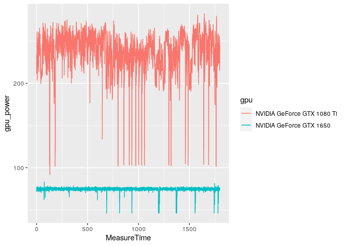
急にパワーが落ちるのは面白いですが、それは誤りではありません。 チェックポイントのロード、崖からの転落、シネマティックスのロードなどに対応するものです。このような短い時間では、グラフィックカードはハードに動作する必要がないため、それほど多くの電力を必要としないのです。
ggplot(doom_data, aes(x = MeasureTime, y = gpu_temperature, color = gpu)) +
  geom_line()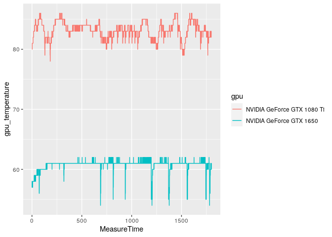
性能の低いカードであるGTX 1650は、チェックポイントの読み込みに対応する温度の低下が大きくなっています。これは、ヒートシンクの熱容量が低く、GTX 1080 Tiに搭載されたアルミニウムのヘットジャンクよりもずっと早く冷却されるためと思われます。
# Technically there may be a small delay until the gpu-die heats up and
# the current temperature of the heatsink may also affect the gpu temperature
cor.test(gtx_1080_ti_doom$gpu_power, gtx_1080_ti_doom$gpu_temperature)
##
## Pearson's product-moment correlation
##
## data: gtx_1080_ti_doom$gpu_power and gtx_1080_ti_doom$gpu_temperature
## t = 48.622, df = 7071, p-value < 2.2e-16
## alternative hypothesis: true correlation is not equal to 0
## 95 percent confidence interval:
## 0.4828882 0.5178252
## sample estimates:
## cor
## 0.5005605そして、その相関関係を見出すのです。
まとめ
- Rを使ってCapFrameXが保存しているJSONを抽出する方法について見てきました。
- GridDBにテーブルスキーマを作成し、JSONファイルからデータを挿入しました。
- RでGridDBに対してパラメータ付きのクエリを作成するために、
pasteとstr_interpを使用しました。 - GridDBのウィンドウ関数を使うことで、ワークステーションにデータを読み込まないようにしました。
- GridDBからデータを取り出してRで解析してみました。
独自のデータを使用したい場合は、データ抽出の過程で一部調整が必要な場合があります。ここでは、「amd_cpu」と「nvidia_gpu」に特化しているので、もし違う組み合わせの場合は、セレクタの名前を変更するか、任意の組み合わせで動作するようにする必要があります。 そして、Githubで共有します。