Exploring Ocean Biodiversity using GridDB and Python
Introduction
Modern Ecological Research is largely data-driven, with actionable insights and decisions made using massive, complex datasets. As timely decision-making is key to real-world research initiatives, the analysis needs to be conducted more quickly yet reliably. The chosen database should support low latency and scale to increased data volumes. GridDB Cloud is one such database that performs in-memory processing, delivering fast, scalable, and resilient performance under heavy workloads. In-memory processing ensures that most data is processed in RAM, reducing disk I/O and enabling faster query responses. In addition, its distributed design allocates data across multiple nodes, enabling parallel query execution and ensuring resilience in the event of node failures. Together, these features make GridDB well-suited to handling large-scale ecological datasets and building scalable applications based on them.
GridDB is built on a key–container data model, where data is stored in containers similar to tables in relational databases. In addition, GridDB provides ACID compliance, ensuring reliable transactions even as workloads scale. While GridDB supports both generic and time-series data, it provides native time-series support with automatic indexing, making it suitable for high-volume telemetry-based applications. That being said, its support for generic non–time–series data is robust as well. Collection containers offer fast ingestion, loading large datasets within seconds. Collections also run SQL‑like queries enabling the use of joins and aggregations. Refer to this resource to learn more about GridDB's architecture .
Pre-requisites
Loading Libraries
#File system and I/O operations
import os
from io import BytesIO
# Data manipulation
import pandas as pd
import numpy as np
from IPython.display import Image

# Time functions
import math
import time
from datetime import datetime, timedelta

# Data Gathering
import requests
import zipfile

#Encoding and Serialization
import base64
import json

#Debugging
import http
http.client.HTTPConnection.debuglevel = 0

#Visualization Libraries
import plotly.graph_objects as go
import plotly.express as px

# Mention your working directory
os.chdir("C:\\Users\\XX")

## Dataset Libraries
from pyobis import dataset
from pyobis import occurrences
About the Dataset
The dataset is obtained from the Ocean Biodiversity Information System (OBIS), a global, open-access biodiversity data ecosystem offering datasets for analysis. We use the dataset 'Observatoire Pelagis aerial surveys 2002-2021' compiled by Van Canneyt, O. and H. Peltie (2022, OBIS-SEAMAP, Version 2.0.0), which is publicly available at https://doi.org/10.82144/436ef8df. We use the 'pyobis' library to fetch the dataset records. This library is covered under the MIT license and can be found here - https://github.com/iobis/pyobis/blob/main/LICENS.
We use the code snippet below to query OBIS metadata and narrow the results to datasets matching a specific keyword. Here, we filter for datasets that include ‘Pelagis’ in their metadata.
query = dataset.search(q="Pelagis")
metadata = query.execute()
ds = metadata['results'][0] #examining the data list object to get the metadata column names like dataset_id
#The metadata for id is dataset_id
print("dataset_id:",ds['id']) #dataset_id
print("dataset_title:",ds['title'])
#print(ds['citation'])
2026-01-16 17:42:41 - pyobis.cache.cache - INFO - Cache initialized at C:\Users\mg_su\AppData\Local\pyobis
dataset_id: 2101d4c5-c20b-49c0-a44b-3d6484c4c891
dataset_title: Observatoire Pelagis aerial surveys 2002-2021
We query the dataset records from the 'occurrences' module in pyobis, using the above dataset_id.
Importing Data Files
#Getting occurrences (data records) from this dataset
dataset_id = "2101d4c5-c20b-49c0-a44b-3d6484c4c891"
query = occurrences.search(datasetid=dataset_id, size=20000)
data = query.execute()
pelagis_df = pd.DataFrame(data)
pd.set_option("display.max_columns", None); pelagis_df.head(n=2)
2026-01-14 23:56:04 - pyobis.cache.cache - INFO - Cache initialized at C:\Users\mg_su\AppData\Local\pyobis
2026-01-14 23:56:04 - pyobis.obisutils - INFO - 20000 to be fetched. Estimated time =0.2940223026275634630 seconds
2026-01-14 23:56:04 - pyobis.obisutils - INFO - Fetching: [█████████████████████████████████████████████████..................................................] 10000/20000
2026-01-14 23:56:04 - pyobis.cache.cache - INFO - Cache initialized at C:\Users\mg_su\AppData\Local\pyobis
2026-01-14 23:56:27 - pyobis.obisutils - INFO - Fetching: [███████████████████████████████████████████████████████████████████████████████████████████████████] 20000/20000
2026-01-14 23:56:27 - pyobis.cache.cache - INFO - Cache initialized at C:\Users\mg_su\AppData\Local\pyobis
2026-01-14 23:56:45 - pyobis.obisutils - INFO - Fetching: [████████████████████████████████████████████████████████████████████████████████████████████████████] 20000/20000
2026-01-14 23:56:45 - pyobis.cache.cache - INFO - Cache initialized at C:\Users\mg_su\AppData\Local\pyobis
2026-01-14 23:56:46 - pyobis.obisutils - INFO - Fetched 20000 records.
| associatedReferences | basisOfRecord | bibliographicCitation | brackish | catalogNumber | class | classid | collectionCode | coordinatePrecision | datasetID | datasetName | dateIdentified | date_end | date_mid | date_start | date_year | day | decimalLatitude | decimalLongitude | eventDate | family | familyid | footprintWKT | genus | genusid | geodeticDatum | georeferencedDate | identificationRemarks | infraorder | infraorderid | infraphylum | infraphylumid | institutionCode | kingdom | kingdomid | license | marine | megaclass | megaclassid | modified | month | nomenclaturalCode | occurrenceID | occurrenceRemarks | occurrenceStatus | order | orderid | ownerInstitutionCode | phylum | phylumid | recordNumber | rightsHolder | scientificName | scientificNameAuthorship | scientificNameID | species | speciesid | specificEpithet | subclass | subclassid | suborder | suborderid | subphylum | subphylumid | superfamily | superfamilyid | taxonRank | taxonRemarks | taxonomicStatus | type | verbatimEventDate | vernacularName | waterBody | year | id | dataset_id | node_id | dropped | absence | originalScientificName | aphiaID | flags | bathymetry | shoredistance | sst | sss | superclass | superclassid | wrims | infraspecificEpithet | subspecies | subspeciesid | infraclass | infraclassid | parvphylum | parvphylumid | unaccepted | category | gigaclass | gigaclassid | superorder | superorderid | subfamily | subfamilyid | |
|---|---|---|---|---|---|---|---|---|---|---|---|---|---|---|---|---|---|---|---|---|---|---|---|---|---|---|---|---|---|---|---|---|---|---|---|---|---|---|---|---|---|---|---|---|---|---|---|---|---|---|---|---|---|---|---|---|---|---|---|---|---|---|---|---|---|---|---|---|---|---|---|---|---|---|---|---|---|---|---|---|---|---|---|---|---|---|---|---|---|---|---|---|---|---|---|---|---|---|---|---|---|---|---|---|
| 0 | [{"crossref":{"citeinfo":{"origin":"Halpin, P.... | HumanObservation | [{"crossref":{"citeinfo":{"origin":"Halpin, P.... | True | 1404_125859 | Mammalia | 1837.0 | 1404 | 1e-06 | 1404 | Observatoire Pelagis aerial surveys 2002-2021 | 2018-05-04 | 1525392000000 | 1525392000000 | 1525392000000 | 2018 | 4 | 1.991593 | 51.298868 | 2018-05-04 | Phocoenidae | 136984.0 | POINT(51.298868 1.991593) | Phocoena | 137031.0 | EPSG:4326 | 2018-05-04 | Identification Type:Visual sighting | Cetacea | 2688.0 | Gnathostomata | 1828.0 | PELAGIS | Animalia | 2 | http://creativecommons.org/licenses/by-nc/4.0/ | True | Tetrapoda | 1831.0 | 2022-01-18 19:37:34 | 5 | WoRMS LSID | 1404_125859 | Visual; plane | present | Cetartiodactyla | 370511.0 | PELAGIS | Chordata | 1821 | 1404_125859 | PELAGIS | Phocoena phocoena | (Linnaeus, 1758) | urn:lsid:marinespecies.org:taxname:137117 | Phocoena phocoena | 137117.0 | phocoena | Theria | 380416.0 | Cetancodonta | 370545.0 | Vertebrata | 146419.0 | Odontoceti | 148723.0 | Species | Taxon recorded as "Phocoena phocoena" by the p... | valid | Event | 2018-05-04 00:00:00 | Harbor porpoise | Global | 2018 | 00000e20-1e69-4620-94bd-bfbbcfacdc6b | 2101d4c5-c20b-49c0-a44b-3d6484c4c891 | [573654c1-4ce7-4ea2-b2f1-e4d42f8f9c31] | False | False | Phocoena phocoena | 137117 | [NO_DEPTH] | 5109.0 | 462157 | 27.73 | 35.35 | NaN | NaN | NaN | NaN | NaN | NaN | NaN | NaN | NaN | NaN | NaN | NaN | NaN | NaN | NaN | NaN | NaN | NaN |
| 1 | [{"crossref":{"citeinfo":{"origin":"Halpin, P.... | HumanObservation | [{"crossref":{"citeinfo":{"origin":"Halpin, P.... | True | 1404_23396 | Aves | 1836.0 | 1404 | 1e-06 | 1404 | Observatoire Pelagis aerial surveys 2002-2021 | 2009-12-15 | 1260835200000 | 1260835200000 | 1260835200000 | 2009 | 15 | -14.206220 | 46.992690 | 2009-12-15 | Laridae | 136988.0 | POINT(46.99269 -14.20622) | NaN | NaN | EPSG:4326 | 2009-12-15 | Identification Type:Visual sighting | NaN | NaN | Gnathostomata | 1828.0 | PELAGIS | Animalia | 2 | http://creativecommons.org/licenses/by-nc/4.0/ | True | Tetrapoda | 1831.0 | 2022-01-18 19:37:34 | 12 | WoRMS LSID | 1404_23396 | Visual; plane | present | Charadriiformes | 2682.0 | PELAGIS | Chordata | 1821 | 1404_23396 | PELAGIS | Laridae | NaN | urn:lsid:marinespecies.org:taxname:136988 | NaN | NaN | NaN | NaN | NaN | NaN | NaN | Vertebrata | 146419.0 | NaN | NaN | Family | Taxon recorded as "Sterna dougalii / bergii…" ... | valid | Event | 2009-12-15 00:00:00 | Gulls | Global | 2009 | 00002a85-f97b-469e-845e-47a09f6fef1c | 2101d4c5-c20b-49c0-a44b-3d6484c4c891 | [573654c1-4ce7-4ea2-b2f1-e4d42f8f9c31] | False | False | Laridae | 136988 | [NO_DEPTH] | 2169.0 | 71134 | 27.97 | 34.75 | Reptilia | 1838.0 | NaN | NaN | NaN | NaN | NaN | NaN | NaN | NaN | NaN | NaN | NaN | NaN | NaN | NaN | NaN | NaN |
Subsetting the Dataset
We subset the dataset to specific columns of interest.
#pelagis_df.columns.to_list()
#We pick the ones that are relevant to our use case
columns_considered = [
 "eventDate",
 "occurrenceID",
 "scientificName",
 "genus",
 "species",
 "aphiaID",
 "family",
 "class",
 "vernacularName",
 "dateIdentified",
 "bathymetry",
 "shoredistance",
 "sst",
 "sss",
 "marine",
 "brackish",
 "absence",
 "flags",
 "waterBody",
 "occurrenceStatus"
]
pelagis_df_final = pelagis_df[columns_considered]

#Standardizing Column Datatypes
pelagis_df_final['flags'] = pelagis_df_final['flags'].astype(str)
pelagis_df_final['brackish'] = pelagis_df_final['brackish'].astype(str)
We will use the 'pelagis_df_final' for container creation and for row registration in GridDB. But before we get started, let's connect to the GridDB instance.
Connecting to GridDB
GridDB can be accessed using different interfaces depending on your environment. The most common options include the GridDB WebAPI for HTTP requests, JayDeBeAPI for JDBC connectivity from Python, and native GridDB client libraries for Java, C, and Python. In this case, we use the WebAPI for connecting to the GridDB Cloud instance. We begin configuring the http request by setting base_url and the request header.
username = "XX" # Provide your GridDB credentials here
password =   "XX"
credentials = f"{username}:{password}"
encoded_credentials = base64.b64encode(credentials.encode()).decode()
#print(f"Encoded credentials: Basic {encoded_credentials}")
#Construct an object to hold the request headers (ensure that you replace the XXX placeholder with the correct value that matches the credentials for your GridDB instance)
#header_obj = {"Authorization":"Basic {EncodedAuthorizationToken}","Content-Type":"application/json; charset=UTF-8","User-Agent":"PostmanRuntime/7.29.0"}

header_obj = {
    "Authorization": f"Basic {encoded_credentials}",  # Add encoded credentials here
    "Content-Type": "application/json",  # Optional; depends on API requirements
    "charset": "UTF-8",
    "User-Agent":"PostmanRuntime/7.29.0"
}

#Construct the base URL based on your GridDB cluster you'd like to connect to (ensure that you replace the placeholders in the URL below with the correct values that correspond to your GridDB instance)
base_url = https://[host]:[port]/griddb/v2/[clustername]/dbs/[database_name]
Creating the Container
Below are some utility functions for facilitating container creation in GridDB. The function 'map_dtype_to_griddb()' maps the Pandas Dataframe data types to the corresponding data types in GridDB. The function 'generate_griddb_data_obj()' helps generate the container structure for container creation. GridDB supports two types of containers namely Collections and TimeSeries containers. TimeSeries containers are primarily used for datasets involving IoT and telemetry data whereas Collections are for more general purpose storage and analysis. Timeseries containers expect the timestamp column to be in the ISO 8601 format ("YYYY-MM-DDThh:mm:ss.SSSZ") so that they can be indexed efficiently. This, in turn, accelerates retrieval when querying large telemetry datasets using TQL (TimeSeries Query Language). However, collection containers have no such requirements. For this blog, we work with a Collection container. To learn more on GridDB's key-container model and the container types, refer to this official GridDB resource .
def map_dtype_to_griddb(dtype):
 # Maps Pandas data types to GridDB data types.
    if pd.api.types.is_integer_dtype(dtype):
        return "INTEGER"
    elif pd.api.types.is_float_dtype(dtype):
        return "DOUBLE"
    elif pd.api.types.is_bool_dtype(dtype):
        return "BOOL"
    ##elif pd.api.types.is_datetime64_any_dtype(dtype):
        ##return "LONG"  # GridDB stores timestamps as LONG
    elif pd.api.types.is_datetime64_any_dtype(dtype):
        return "TIMESTAMP"
    else:
        return "STRING"
def generate_griddb_data_obj(df, container_name="MyContainer", container_type="COLLECTION", rowkey=False):
    #Generates a GridDB container data object for API request.
    columns = []
    for col in df.columns:
        griddb_type = map_dtype_to_griddb(df[col].dtype)
        columns.append({"name": col, "type": griddb_type})

    data_obj = {
        "container_name": container_name,
        "container_type": container_type,
        "rowkey": rowkey,
        "columns": columns
    }

    return data_obj
data_obj = generate_griddb_data_obj(pelagis_df_final, container_name="pelagis")

#Set up the GridDB WebAPI URL
url = base_url + 'containers'

#Invoke the GridDB WebAPI with the headers and the request body
x = requests.post(url, json = data_obj, headers = header_obj)
#x.text
''
Row Registration
In GridDB, rows can be ingested in bulk or in batches. Batch insertion is more efficient for large datasets and helps speed up data ingestion. For our example, we ingested 20,000 rows which took about 9 seconds, which is roughly 2,200 rows per second.
#Setup the URL to be used to invoke the GridDB WebAPI to register rows in the container created previously
url = base_url + 'containers/pelagis/rows'
print(url)
batch_size = 5000
total_rows = len(pelagis_df_final)
total_batches = math.ceil(total_rows / batch_size)

print(f"Starting ingestion of {total_rows:,} rows in {total_batches} batches of {batch_size} each...")
start_time = time.time()

for i in range(total_batches):
    start_idx = i * batch_size
    end_idx = min((i + 1) * batch_size, total_rows)
    batch_df = pelagis_df_final.iloc[start_idx:end_idx]
    batch_json = batch_df.to_json(orient='values')

    try:
        print(url)
        response = requests.put(url, headers=header_obj, data=batch_json)
        elapsed = time.time() - start_time

        if response.status_code in [200, 201]:
            print(f" Batch {i+1}/{total_batches} | Rows {start_idx}-{end_idx-1} | "
                  f"Time elapsed: {elapsed:.1f}s")
        else:
            print(f" Batch {i+1}/{total_batches} FAILED "
                  f"(HTTP {response.status_code}) - {response.text[:150]}")

    except Exception as e:
        print(f" Batch {i+1}/{total_batches} ERROR: {e}")

print(f"\n Ingestion completed in {time.time() - start_time:.1f} seconds.")
Querying Data
GridDB supports SQL queries for collection containers; and both SQL and TQL (TimeSeries Query Language) for timeseries containers. Refer to the official SQL reference to learn more.
Top 10 Most Observed Species by Year
In the query below, we aim to extract the top 10 species based on the year they were identified. For this, we use standard timestamp functions and aggregation functions as shown below. Refer to this resource to learn more on GridDB's time functions .
sql_query1 = ("""
            SELECT p.genus,
            p.class,
            EXTRACT(YEAR, TIMESTAMP(p.dateIdentified)) AS year_identified,
            p.vernacularName,
            count(DISTINCT p.occurrenceID) as num_occurrences
            FROM pelagis p
            GROUP BY 1,2,3,4
            HAVING COUNT(DISTINCT p.occurrenceID) > 0
            ORDER BY 5 DESC
            """)
#Setup the URL to be used to invoke the GridDB WebAPI to retrieve data from the container
url = base_url + 'sql'

# Construct the request body
request_body = json.dumps([
    {
        "type": "sql-select",
        "stmt": sql_query1
    }
])

# Disable HTTP debugging
http.client.HTTPConnection.debuglevel = 0

#Invoke the GridDB WebAPI
data_req1 = requests.post(url, data=request_body, headers=header_obj)

#Process the response received and construct a Pandas dataframe with the data from the response
myJson = data_req1.json()
occurrences_df = pd.DataFrame(myJson[0]["results"], columns=[myJson[0]["columns"][0]["name"], myJson[0]["columns"][1]["name"], myJson[0]["columns"][2]["name"], myJson[0]["columns"][3]["name"], myJson[0]["columns"][4]["name"]])
occurrences_df['year_identified'] = occurrences_df['year_identified'].astype(str)
fig = px.bar(occurrences_df, x="year_identified", y="num_occurrences", color="genus", title="Most Observed Species by Year",text="num_occurrences")
fig.update_traces(textposition='inside')
fig.show()
Insight(s): The years 2011 and 2014 have had the most sightings, with different genera being identified during these years. Larus seems to have been identified across multiple years from 2011 to 2018 whereas Onychoprion sightings have been the highest around 2010. This suggests that different bird genera have distinct patterns of occurrence over time.
Distribution of the Sea Surface Temperature and Salinity Over the Years
In the next query, we aim to identify the average surface temperature and average surface salinity. This helps us understand the preferences of different creatures that are identified in marine waters. We use standard aggregation functions for this. Check out the GridDB resource to learn more on the aggregation functions supported.
sql_query2 = ("""
                SELECT
                EXTRACT(YEAR, TIMESTAMP(p.eventDate)) AS year,
                AVG(p.sst) AS avg_sst,
                AVG(p.sss) AS avg_sss
                FROM pelagis p
                WHERE p.occurrenceStatus = 'present'
                GROUP BY year
                ORDER BY year
                """)
#Setup the URL to be used to invoke the GridDB WebAPI to retrieve data from the container
url = base_url + 'sql'

# Construct the request body
request_body = json.dumps([
    {
        "type": "sql-select",
        "stmt": sql_query2
    }
])

# Disable HTTP debugging
http.client.HTTPConnection.debuglevel = 0

#Invoke the GridDB WebAPI
data_req2 = requests.post(url, data=request_body, headers=header_obj)

#Process the response received and construct a Pandas dataframe with the data from the response
myJson = data_req2.json()
avg_metrics_df = pd.DataFrame(myJson[0]["results"], columns=[myJson[0]["columns"][0]["name"], myJson[0]["columns"][1]["name"], myJson[0]["columns"][2]["name"]])
fig = px.line(
    avg_metrics_df,
    x='year',
    y=['avg_sst','avg_sss'],
    markers=True,  # shows points
    labels={'value':'Measurement','variable':'Parameter'},
    title='Distribution of SSS and SST Over The Years'
)

fig.show()
Insight(s): The average Sea Surface Temperature seems to have fluctuated quite a bit, with sharp peaks around 2008, 2015, 2017 and 2018. The sea surface salinity seems to follow a fairly steady trend, with a slight fluctuation in 2019. These readings can influence the presence of marine organisms greatly, as some organisms might prefer warmer and more saline waters, whereas some would prefer colder waters. Let's delve more into this in later queries.
Observations by Depth Levels
In this query, we create a new category called depth range (depth level) using CASE WHEN logic, based on the 'bathmetry' column. Our objective here is to find if depth has anything to do with increased occurrence of species (sightings). To learn more about the CASE logic, refer to the resource here.
sql_query3 = ("""SELECT
            CASE
                WHEN p.bathymetry < 500 THEN 'Shallow (<500m)'
                WHEN p.bathymetry BETWEEN 500 AND 1500 THEN 'Mid-depth (500-1500m)'
                ELSE 'Deep (>1500m)'
            END AS depth_range,
            COUNT(p.occurrenceID) AS num_observations
            FROM pelagis p
            WHERE p.occurrenceStatus = 'present'
            GROUP BY depth_range
            ORDER BY 2 DESC """)
#Setup the URL to be used to invoke the GridDB WebAPI to retrieve data from the container
url = base_url + 'sql'

# Construct the request body
request_body = json.dumps([
    {
        "type": "sql-select",
        "stmt": sql_query3
    }
])

# Disable HTTP debugging
http.client.HTTPConnection.debuglevel = 0

#Invoke the GridDB WebAPI
data_req3 = requests.post(url, data=request_body, headers=header_obj)

#Process the response received and construct a Pandas dataframe with the data from the response
myJson = data_req3.json()
occurrences_by_depth_range_df = pd.DataFrame(myJson[0]["results"], columns=[myJson[0]["columns"][0]["name"], myJson[0]["columns"][1]["name"]])
fig = px.bar(occurrences_by_depth_range_df, x='depth_range', y='num_observations', text='num_observations', title ='Sightings by Depth Levels'
)

fig.update_traces(textposition='inside')

fig.show()
C:\Users\mg_su\conda\anaconda3\Lib\site-packages\kaleido\_sync_server.py:11: UserWarning:


Warning: You have Plotly version 5.22.0, which is not compatible with this version of Kaleido (1.2.0).

This means that static image generation (e.g. `fig.write_image()`) will not work.

Please upgrade Plotly to version 6.1.1 or greater, or downgrade Kaleido to version 0.2.1.
Insight(s): We see that most marine life seems to have been sighted in shallow waters, followed by some in deep waters. Mid-depth sightings seem to be very low, which could either be due to the fact that they are undersurveyed (due to technical constraints); or that fewer species inhabit this zone.
Observations by Shore Distance and Brackishness
In the next query, we create a new bucket called 'Shore_band' based on the shoredistance column. We also look at brachishness to see how the two aspects relate to sightings.
sql_query4 = ("""SELECT
              CASE
              WHEN shoredistance < 10 THEN 'Very Near Shore (<10km)'
              WHEN shoredistance BETWEEN 10 AND 50 THEN 'Near Shore (10–50km)'
              WHEN shoredistance BETWEEN 50 AND 200 THEN 'Offshore (50–200km)'
              ELSE 'Far Offshore (>200km)'
              END AS shore_band,
              brackish,
              COUNT(occurrenceID) AS num_occurrences
              FROM pelagis
              WHERE brackish != 'nan'
              GROUP BY 1, 2
              ORDER BY num_occurrences DESC""")
#Setup the URL to be used to invoke the GridDB WebAPI to retrieve data from the container
url = base_url + 'sql'

# Construct the request body
request_body = json.dumps([
    {
        "type": "sql-select",
        "stmt": sql_query4
    }
])

# Disable HTTP debugging
http.client.HTTPConnection.debuglevel = 0

#Invoke the GridDB WebAPI
data_req4 = requests.post(url, data=request_body, headers=header_obj)

#Process the response received and construct a Pandas dataframe with the data from the response
myJson = data_req4.json()
occurrences_by_shore_distance_df = pd.DataFrame(myJson[0]["results"], columns=[myJson[0]["columns"][0]["name"], myJson[0]["columns"][1]["name"], myJson[0]["columns"][2]["name"]])
fig = ff.create_table(occurrences_by_shore_distance_df)
fig.show()
Insight(s): We see that majority of the organisms are found far away from the shore and in coastal mixing zones which is a mix of fresh water and salt water (brackish = True). It is also evident that almost no species prefers being in fresh wster in an offshore band of 50-200 km. Some, however prefer fresh water but like to be in the far offshore band of more than 200 km.
Comparing Surface Metrics to Sightings
Here, we calculate the average surface temperature and surface salinity to sightings while only considering sightings greater than 10. We also perform some null handling using IFNULL(). To learn more about special handling functions supported by GridDB, refer to this resource .
sql_query5 = """SELECT
                IFNULL(p.vernacularName,'Not Specified') as VernacularName,
                AVG(p.sst) AS avg_sst,
                AVG(p.sss) AS avg_sss,
                COUNT(p.occurrenceID) AS num_occurrences
                FROM pelagis p
                WHERE p.genus IS NOT NULL
                GROUP BY p.vernacularName
                HAVING COUNT(p.occurrenceID) > 10
                ORDER BY num_occurrences DESC
                LIMIT 15
                """
#Setup the URL to be used to invoke the GridDB WebAPI to retrieve data from the container
url = base_url + 'sql'

# Construct the request body
request_body = json.dumps([
    {
        "type": "sql-select",
        "stmt": sql_query5
    }
])

# Disable HTTP debugging
http.client.HTTPConnection.debuglevel = 0

#Invoke the GridDB WebAPI
data_req5 = requests.post(url, data=request_body, headers=header_obj)

#Process the response received and construct a Pandas dataframe with the data from the response
myJson = data_req5.json()
avg_metrics_df = pd.DataFrame(myJson[0]["results"], columns=[myJson[0]["columns"][0]["name"], myJson[0]["columns"][1]["name"], myJson[0]["columns"][2]["name"], myJson[0]["columns"][3]["name"]])
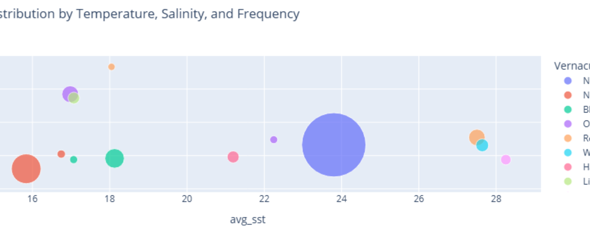
fig = px.scatter(
    avg_metrics_df,
    x="avg_sst",
    y="avg_sss",
    size="num_occurrences",
    color="VernacularName",
    hover_name="VernacularName",
    title="Species Distribution by Temperature, Salinity, and Frequency",
    size_max=60
)
fig.show()
Insight(s): The majority of the creatures (7952 occurrences) identified seem to prefer highly saline waters having a surface salinity of around 35 PSU. Majority of them prefer lower surface temperatures. However, we do not have the vernacular names for these species. Among the identified species having vernacular names, the Northern Gannets, The Litte Gull and Ocean Sunfish seem to have been the most identified in cold water bodies.
We create another plot to identify warm water species and cold water species, along with the ones that prefer higher salinities.
melted = avg_metrics_df.melt(
    id_vars="VernacularName",
    value_vars=["avg_sst", "avg_sss"],
    var_name="metric",
    value_name="value"
)

fig = px.bar(
    melted,
    x="VernacularName",
    y="value",
    color="metric",
    barmode="group",
    title="Average Sea Temperature and Salinity by Species"
)
fig.show()
Insight(s): Most of the species live in typical open-ocean salinity conditions between 34 and 35 PSU. The Yellow-legged gull seems to prefer more saline waters than other species (37.6 PSU). Similarly, ocean sunfish seems to like high saline conditions (36.8 PSU). White-trailed tropicbirds, the Red-footed booby and the Angel tern seem to prefer warmer waters (Surface Temperatures of 27 to 28 degree Celsius).
Concluding Remarks
This walkthrough demonstrates how GridDB can be used to wrangle real‑world ecological data with minimal overhead. We ingested the data into GridDB Cloud and used GridDB SQL to effectively explore and visualize patterns and trends in marine sightings. This simple exploration opens doors to deeper investigations. There is plenty of room for more intricate analysis such as analyzing the behavior of a genus in a specific habitat or investigating why some genus sightings dropped over time. Using GridDB and Python, we could create statistical or ML models to forecast species occurrences or develop real-time monitoring dashboards of sightings. For real-world datasets that are large, GridDB's parallel processing and distributed architecture can help scale analysis without slowing down insights.
If you have any questions about the blog, please create a Stack Overflow post here https://stackoverflow.com/questions/ask?tags=griddb .
Make sure that you use the “griddb” tag so our engineers can quickly reply to your questions.