The R programming language is a favorite of data scientists for conducting statistical analysis of datasets. Generally an analysis of large datasets benefit greatly from having a fast database backing the data — that’s where GridDB comes in.
For this article, we will be looking to ingest a large dataset via R, and then with the large dataset in place, we will run a variety of SQL queries to see what kind of information we can glean from the dataset. Lastly, because the R programming language excels at graphing our data, we will try to plot our results with gplot.
Table of Contents
- Getting Started
- Picking a Dataset
- Ingest Play-by-Play Data via hoopR
- Analyzing Play by Play Data
- Other Sorts Ideas for Analysis
- Conclusion
Getting Started
To follow along, you can clone the repo with the following:
$ git clone -b r_analysis git@github.com:griddbnet/Project.gitPrerequisites
You will need
- GridDB
- R
- An R IDE like RStudio
Sequence of Operations
To run this you will need to accomplish the following:
- Clone the repo
-
Install the necessary libraries:
- install.packages(“RJDBC”,dep=TRUE)
- install.packages(“rJava”)
- install.packages(“hoopR”)
- install.packages(“nflreadr”)
- install.packages(“devtools”, dep=TRUE)
- devtools::install_github(“abresler/nbastatR”)
- install.packages(‘stringr’)
- install.packages(‘dplyr’)
- install.packages(‘ggplot2’)
- install.packages(‘lubridate’)
- install.packages(‘ggalt’)
-
Run the Ingest code (
ingest.R) -
Run the querying code (
query.R)
Picking a Dataset
Picking an extremely large dataset can lead us down many paths — we are, after all, in the era of big data. For this article, we have opted to use go in a slightly-off-kilter direction: sports. Using the hoopR library, we can ingest play-by-play data from all NBA seasons starting from 2002 until the most recent season. In this case, ingesting all of the seasons did not seem necessary, so we opted to simply ingest the latest season and conduct our analysis from there.
Ingest Play-by-Play Data via hoopR
To ingest our dataset, we first need to connect to our running GridDB server.
Connecting to GridDB via JDBC
As mentioned before, we will utilize JDBC to connect to our server. Luckily, there is a package which allows for the programming language R to connect directly via JDBC called RJDBC. Using this package, we can simply enter our JDBC credentials and create a connection with GridDB. Once that connection is made, we can use the DBI connection to make sql queries to our GridDB instance.
To make the connection, we must of course import the appropriate library and then enter our credentials, including the GridDB JDBC file.
library(RJDBC)

drv <- JDBC("com.toshiba.mwcloud.gs.sql.Driver",
            "/usr/share/java/gridstore-jdbc-5.0.0.jar")
             #identifier.quote = "`")

conn <- dbConnect(drv, "jdbc:gs://127.0.0.1:20001/myCluster/public", "admin", "admin")
If all of your details are correct, the conn variable will now be a DBI connection to GridDB. With this done, we can move on to ingesting our dataset.
Ingesting Data via JDBC
To accomplish ingesting the play-by-play data, we will look to hoopR’s built-in functions which attempts to do all the work for us. The library’s function load_nba_pbp looks to be exactly what is needed: it accepts a DBI connection as one of its parameters and will load a specific year of data into our DB connection. From looking at the source code, we can see that the data is available to us in .csv and .rds file format directly from one of the hoopR’s publically available GitHub repositories.
So to ingest, we will load in the file directly from GitHub and ingest the data, line by line until it is finished. Using the RJDBC API allows us to simply call .dbWritetable and it will handle creating our SQL statements for us, including creating the table.
loader <- rds_from_url
urls <- paste0("https://raw.githubusercontent.com/sportsdataverse/hoopR-data/main/nba/pbp/rds/play_by_play_2022.rds")

p <- NULL

out <- lapply(urls, progressively(loader, p))
out <- rbindlist_with_attrs(out)

out$type_abbreviation <- NULL

for (i in 1:nrow(out)) {
  RJDBC::dbWriteTable(conn, "nba_pbp_2022", out[i, ], append = TRUE )
}
That’s the entirety of our ingest script; it simply reads in the file directly from GitHub and then goes line by line, ingesting until finished, roughly 600,000 lines of data. Once it is done, any aspects of the latest 2022 NBA season can be analyzed with some queries.
Analyzing Play by Play Data
To analyze the data, we can simply form SQL queries to return data we want to look at. First, let’s take a look at the all of the columns included in the dataset:
Columns:
No  Name                  Type            CSTR  RowKey
------------------------------------------------------------------------------
 0  shooting_play         STRING
 1  sequence_number       STRING
 2  period_display_value  STRING
 3  period_number         INTEGER
 4  home_score            INTEGER
 5  coordinate_x          INTEGER
 6  coordinate_y          INTEGER
 7  scoring_play          STRING
 8  clock_display_value   STRING
 9  team_id               STRING
10  type_id               STRING
11  type_text             STRING
12  away_score            INTEGER
13  id                    DOUBLE
14  text                  STRING
15  score_value           INTEGER
16  participants_0_athlete_id  STRING
17  participants_1_athlete_id  STRING
18  participants_2_athlete_id  STRING
19  season                INTEGER
20  season_type           INTEGER
21  game_id               INTEGER
22  away_team_id          INTEGER
23  away_team_name        STRING
24  away_team_mascot      STRING
25  away_team_abbrev      STRING
26  away_team_name_alt    STRING
27  home_team_id          INTEGER
28  home_team_name        STRING
29  home_team_mascot      STRING
30  home_team_abbrev      STRING
31  home_team_name_alt    STRING
32  home_team_spread      DOUBLE
33  game_spread           DOUBLE
34  home_favorite         STRING
35  game_spread_available  STRING
36  qtr                   INTEGER
37  time                  STRING
38  clock_minutes         INTEGER
39  clock_seconds         DOUBLE
40  half                  STRING
41  game_half             STRING
42  lag_qtr               DOUBLE
43  lead_qtr              DOUBLE
44  lag_game_half         STRING
45  lead_game_half        STRING
46  start_quarter_seconds_remaining  INTEGER
47  start_half_seconds_remaining  INTEGER
48  start_game_seconds_remaining  INTEGER
49  game_play_number      INTEGER
50  end_quarter_seconds_remaining  DOUBLE
51  end_half_seconds_remaining  DOUBLE
52  end_game_seconds_remaining  DOUBLE
53  period                INTEGER
To show this information we used the GridDB CLI’s showcontainer command: showcontainer nba_pbp_2022.
Choosing Relevant Datapoints
Though there of course many directions in which we can take our analysis, one of the most visually pleasing datapoints to chart onto a plot is shot makes and misses. It would be even better if we could somehow plot the results of the datapoints onto a plot which resembled an NBA court for proper context. Luckily for us, we can see some columns which can help us with this endeavor, namely: coordinate_x, coordinate_y, score_value, shooting_play, participants_0_athlete_id, and type_id.
Using those columns we can grab the coordinates of a variety of different plays from specific players, from specific games, or from specific teams. Specifically we can see that type_id can correspond to many different event types. For example, we can specifically target Step Back Jump Shot by searching for type_id of 132. For example, as of right now Luka Doncic comes to mind as the step back jumpshot leader, especially with James Harden being hampered by injuries as of late.
To check if this is true, we can simply run a SQL query. To start, let’s run this query in our shell and then we are happy with the data results, we can move to plotting our data onto a plot.
Querying the Dataset
To start, let’s try to get the count of step back attempts by both players. We formulate our SQL query: SELECT COUNT(*) FROM nba_pbp_2022 WHERE shooting_play = 'TRUE' AND participants_0_athlete_id = '3945274' AND type_id = '132'. Here our query is finding all instances where Luka Doncic attempted a step back jump shot — this includes both makes and misses. Running this query shows a blistering 450 attempts from Luka Doncic on step back jumpshots. Although please note that this dataset also includes all of the postseason which of course adds some volume to this metric as he made round 3 of the playoffs.
If we make the same query for James Harden I suspect we see a much smaller total, even though Harden is the player who popularized the move. Let’s run this query: SELECT COUNT(*) FROM nba_pbp_2022 WHERE shooting_play = 'TRUE' AND participants_0_athlete_id = '3992' AND type_id = '132'. And sure enough, we get 349 results, with the last attempt being in a losing effort to the Miami Heat in game 6 of the Eastern Conference SemiFinals.
But what if instead of looking at total attempts, we wanted to know who made more shots of this type? To do so, we can simply add a score_value of 2 or greater in our query: SELECT COUNT(*) FROM nba_pbp_2022 WHERE shooting_play = 'TRUE' AND participants_0_athlete_id = '3945274' AND type_id = '132' AND score_value >= 2. Once we run this query for both players, we see that Harden shot 122/349 on step back shots, while Luka shot 175/450, or better stated that Harden shot ~35% on step back shots compared to Luka’s ~39% on higher volume; perhaps Luka is the new step back king!
Here’s what that chart looks like
Visualizing The Dataset
So now we know that Luka shot better and on more attempts of step back jumpshots. Wouldn’t it be cool to be able to visualize where on the court Luka was attempting and making these shots? As stated before, the play by play data includes coordinates for where a specific event occured. So we can directly query to extract the coordinates for all step back jump shots. Now to plot these values onto something resembling an NBA court.
To accomplish this feat, we can borrow the court made by the ballr library. Once we are able to draw the court with ggplot, we mutate our coordinates to match what the court expects and plot all of the precise locations of the events onto an NBA half court visualization.
queryString <- "select coordinate_x, coordinate_y from nba_pbp_2022 WHERE shooting_play = 'TRUE' AND participants_0_athlete_id = '3945274' AND type_id = '132'"
rs <- dbGetQuery(conn, queryString )

source("https://raw.githubusercontent.com/toddwschneider/ballr/master/plot_court.R")
source("https://raw.githubusercontent.com/toddwschneider/ballr/master/court_themes.R")
plot_court() # created the court_points object we need
court_points <- court_points %>% mutate_if(is.numeric,~.*10)

rs <- rs  %>%  mutate_if(is.numeric,~.*10)
And then of course, the final step will be to plot all of our data points directly onto our court_points
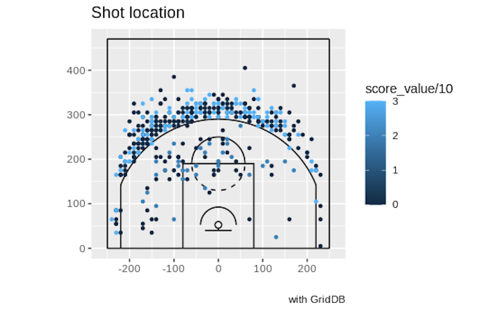
DBcourt <-
  ggplot(rs, aes(x=coordinate_x-250, y=coordinate_y+45)) +
  scale_fill_manual(values = c("#00529b","#cc4b4b"),guide='none')+
  geom_path(data = court_points,
            aes(x = x, y = y, group = desc),
            color = "black")+
  coord_equal()+
  geom_point(aes(fill="TRUE",color=score_value/10),size=1) +
  xlim(-260, 260)+
  labs(title="Shot location",x="",
       y="",
       caption = "with GridDB")

print(DBcourt)
With this snippet of code, we are plotting our coordinates for all of Luka Doncic’s step back jumpers. The makes will be in a brighter shade of blue, and the misses will be nearly black. Because it is 450 data points plotted onto a small court, it is a tad messy but you can get a feel of how he did throughout the season.
Other Sorts of Ideas for Analysis
Of course, analyzing just step back jumpers is only a small sliver of what you can do with this much data at your disposal. You can, for example, also look at made shots in the 4th quarter to try to extrapolate “clutchness”. Really, with this much data, the possibilities are limitless.
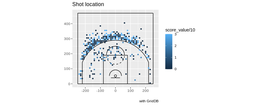
Here are some examples of simple shot charts you could make for different players. First, let’s take a look at all of Steph Curry’s made baskets for the season and then chart it:
queryString <- "select coordinate_x, coordinate_y from nba_pbp_2022 WHERE shooting_play = 'TRUE' AND participants_0_athlete_id = '3975' AND score_value >= 2"
Or let’s try it for Giannis Antetokounmpo:
queryString <- "select coordinate_x, coordinate_y from nba_pbp_2022 WHERE shooting_play = 'TRUE' AND participants_0_athlete_id = '3032977' AND score_value >= 2"
Klay Thompson:
queryString <- "select coordinate_x, coordinate_y from nba_pbp_2022 WHERE shooting_play = 'TRUE' AND participants_0_athlete_id = '6475' AND score_value >= 2"
LeBron James:
queryString <- "select coordinate_x, coordinate_y from nba_pbp_2022 WHERE shooting_play = 'TRUE' AND participants_0_athlete_id = '1966' AND score_value >= 2"
Conclusion
And with that, we have seen how to use GridDB with R and how to query extremely large datasets and to visualize said dataset.