
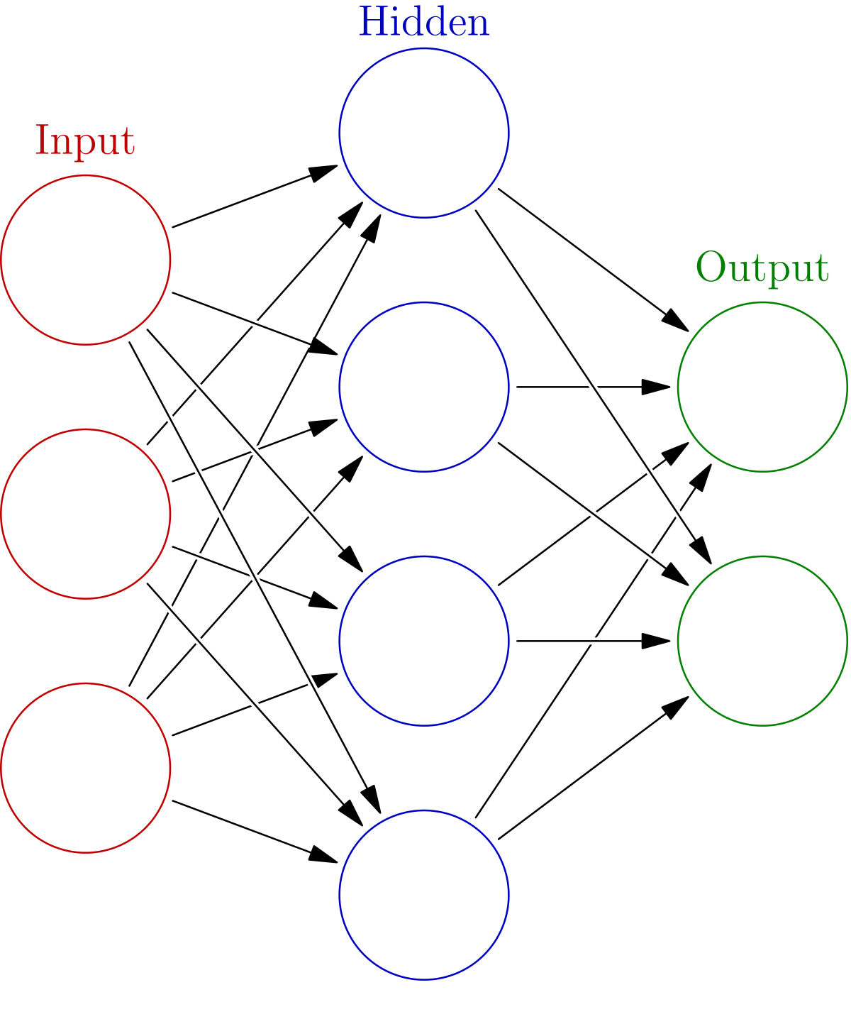
Neural Networks have taken the world of machine learning and predictive modelling in the last 5 years. Neural network have the ability to learn complex relationships in data and have been shown to work for a variety of applications from finance to robotics. Inspired by the human brain, Neural Networks work on the principle of signal transmission from one neuron to the other. Neural networks comprise of mainly three types of node layers — an input layer, one or more hidden layers, and an output layer. Each node is an artificial neuron which connects to another using a nonlinear function and has an associated weight and threshold. The neuron is activated only if the output is above the specified threshold value. This is how the data is passed along to the next layer of the network.
Toshiba GridDB is a highly scalable database optimized for IoT and Big Data. GridDB lets us collect, store and query large amount of data easily. Moreover, GridDB is highly scalable and ensures high reliability, as a result it can server as a great database for neural networks training and inference. Installing GridDB is pretty simple, and is well documented here. To checkout the python-gridDB client please refer to this video.
In this post we will create train a simple neural network based classification model in python with GridDB. We will use Keras, which is an easy-to-use free open source Python library for developing and evaluating deep learning models.
Setup
Let’s setup GridDB first!
Quick setup of GridDB Python Client on Ubuntu 20.04:
-
Install GridDB Download and install the deb from here.
-
Install C client Download and install the Ubuntu from here.
-
Install requirements 1) Swig
wget https://github.com/swig/swig/archive/refs/tags/v4.0.2.tar.gz
tar xvfz v4.0.2.tar.gz
cd swig-4.0.2
./autogen.sh
./configure
make
2) Install python client
wget
https://github.com/griddb/python_client/archive/refs/tags/0.8.4.zip
unzip . 0.8.4.zip
Make sure you have python-dev installed for the corresponding python version. We will use python 3.8 for this post.
3) We also need to point to the correct locations
export CPATH=$CPATH:<python header file directory path>
export LIBRARY_PATH=$LIBRARY_PATH:<c client library file directory path></c></python>
We can also use GridDB with docker as shown here
Python libraries
Next we install the python libraries. Installing matplotlib, numpy, keras, tensorflow and pandas is a simple pip install.
pip install keras
pip install numpy
pip install tensorflow
pip install matplotlib
pip install pandas
Prediction
Step 1: Downloading Dataset
We will use a publicly available dataset from Kaggle. For this post we have picked the mobile price classification. The aim is to classify cellphones into four price categories. Below is the description of the dataset.
| column | description |
|---|---|
| battery_power | Total energy a battery can store in one time measured in mAh |
| blue | Has Bluetooth or not |
| clock_speed | speed at which microprocessor executes instructions |
| dual_sim | Has dual sim support or not |
| fc | Front Camera megapixels |
| four_g | Has 4G or not |
| int_memory | Internal Memory in Gigabytes |
| m_dep | Mobile Depth in cm |
| mobile_wt | Weight of mobile phone |
| n_cores | Number of cores of processor |
| pc | Primary Camera mega pixels |
| px_height | Pixel Resolution Height |
| px_width | Pixel Resolution Width |
| ram | Random Access Memory in MegaBytes |
| sc_h | Screen Height of mobile in cm |
| sc_w | Screen Width of mobile in cm |
| talk_time | longest time that a single battery charge will last when you are |
| three_g | Has 3G or not |
| touch_screen | Has touch screen or not |
| wifi | Has wifi or not |
| price_range | This is the target variable with values of 0(low cost), 1(medium cost), 2(high cost), and 3(very high cost). |
Step 2: Importing Libraries
We first import relevant libraries i.e pandas for loading the dataset, matplotlib for visualisations and tensorflow for the deep learning model.
import tensorflow as tf
import numpy as np
import pandas as pd
from tensorflow import keras
from tensorflow.keras import layers
Step 3: Data Loading and Processing
Loading Data
First we load the data. For this we use the read_csv functionality in pandas. Note that the dataset has the test and train already sperated into two files.
dataframe = pd.read_csv('train.csv')Alternatively, we can use GridDB to get this dataframe.
Feature Encoding
We first encode the data sets into categorical and numeric format. For numeric we will normalize the data and for categorical we will convert the data type. We also create a set of features and remove the target from the set of features.
numeric_feats = ["mobile_wt", "m_dep", "int_memory", "fc", "clock_speed", "talk_time","n_cores", "sc_w", "sc_h", "ram", "px_width","px_height","pc", "battery_power"]

dataframe[numeric_feats] = dataframe[numeric_feats].apply(lambda x: (x - np.mean(x)) / (np.max(x) - np.min(x)))

categorical_feats = ["blue", "four_g", "dual_sim", "wifi", "touch_screen", "three_g","price_range"]
dataframe[categorical_feats] =  dataframe[categorical_feats].astype("category")

features = numeric_feats + categorical_feats
features.remove("price_range")
We can now describe the dataset and check the distribution.
dataframe[numeric_feats].describe()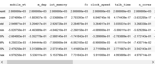
dataframe[categorical_feats].describe()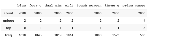
Splitting Data into Validation and Train
We then create a small validation set to test data on while training to make sure we do not overfit on the data. We take 20% of the data as validation set.
val_dataframe = dataframe.sample(frac=0.2, random_state=1337)
train_dataframe = dataframe.drop(val_dataframe.index)

print("Number of training samples:", len(train_dataframe))
print("Number of validation samples:", len(val_dataframe))
Preparing data for Keras
Since this is a multiclass classification problem. We have to convert the target to one-hot encoding. We do that with tf.keras.utils.to_categorical. As keras takes in numpy arrays, we convert the pandas dataframe to numpy.
Y_train = tf.keras.utils.to_categorical(train_dataframe["price_range"], num_classes=4)
Y_val = tf.keras.utils.to_categorical(val_dataframe["price_range"], num_classes=4)

X_train = train_dataframe[features].values
X_val = val_dataframe[features].values
Step 4: Prediction
Next we start the prediction process.
Initializing
We will create a simple model for our prediction. We will add 12 dense layers. Note that we will make the input dimensions 20. Then we add a dropout module that helps with overfitting. Finally w e add a few more hidden layers and then end it with a softmax. The softmax gives us four probability scores for the four classes. We can play around with the model configurations, adding or deleting layers.
# define the keras model
model =  keras.Sequential()
model.add(layers.Dense(12, input_dim=20, activation='relu'))
model.add(layers.Dropout(0.5))
model.add(layers.Dense(8, activation='relu'))
model.add(layers.Dense(4, activation='softmax'))
Training
Next we compile the model. We use the categorical cross entropy as the loss and evaluate it on accuracy. Ideally we can use AUC or any other metric we seem fit.
model.compile(loss='categorical_crossentropy', optimizer='adam', metrics=['accuracy'])Next we train the model for 200 epochs.
num_epochs = 200
history = model.fit(X_train,
                   Y_train,
                   epochs=num_epochs ,
                   validation_data=(X_val, Y_val))
Epoch 1/200
50/50 [==============================] - 0s 2ms/step - loss: 0.1648 - accuracy: 0.9431 - val_loss: 0.2359 - val_accuracy: 0.9125
Epoch 2/200
50/50 [==============================] - 0s 2ms/step - loss: 0.1871 - accuracy: 0.9388 - val_loss: 0.1986 - val_accuracy: 0.9175
Epoch 3/200
....
Epoch 199/200
50/50 [==============================] - 0s 1ms/step - loss: 0.1245 - accuracy: 0.9575 - val_loss: 0.4880 - val_accuracy: 0.8075
Epoch 200/200
50/50 [==============================] - 0s 1ms/step - loss: 0.1267 - accuracy: 0.9600 - val_loss: 0.4585 - val_accuracy: 0.8150Evaluation
Next we plot the loss and the accuracy for the train and validation. Ideally the loss should go down and the accuracy would go up.
history = history.historyimport matplotlib.pyplot as plt
%matplotlib inline
epochs = list(range(num_epochs))
loss = history["loss"]
val_loss = history["val_loss"]
plt.plot(epochs, loss, 'bo', label="Training Loss")
plt.plot(epochs, val_loss, 'b', label="Validation Loss")
plt.title('Training and Validation Loss')
plt.xlabel('Epochs')
plt.ylabel('Loss Value')
plt.legend()
plt.show()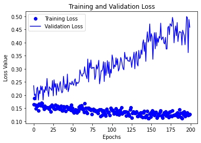
epochs = list(range(num_epochs))
accuracy = history["accuracy"]
val_accuracy = history["val_accuracy"]
plt.plot(epochs, accuracy, 'bo', label="Accuracy")
plt.plot(epochs, val_accuracy, 'b', label="Val Accuracy")

plt.title('Training and Validation Accuracy')
plt.xlabel('Epochs')
plt.ylabel('Loss Value')
plt.legend()
plt.show()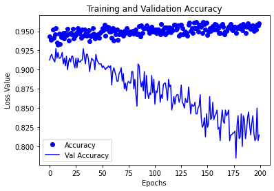
Note that the val accuracy is going down but the tain accuracy is constant this may imply that the model is overfitting. In that case we can either try several strategies: reduce epochs, use a different loss function, argument the data and so on.
Predictions
# evaluate the keras model
test = pd.read_csv('test.csv')
test[numeric_feats] = test[numeric_feats].apply(lambda x: (x - np.mean(x)) / (np.max(x) - np.min(x)))

if "price_range" in categorical_feats:
  categorical_feats.remove("price_range")

test[categorical_feats] =  test[categorical_feats].astype("category")
feats = test[features].values
predictions = model.predict(feats)
predictions = np.argmax(predictions, axis=1)
Finally we load the testing data and predict. Note that keras will return probabilities for each class, so we take the argmax to get the class.
Conclusion
In this article we learnt how to train a simple neural network for a classification task.