Structured Insights from SEC Filings: Leveraging GridDB's NewSQL Interface and RESTful WebAPI
Introduction
GridDB is a high-performance time-series database with a key-container model at its core. GridDB offers two types of containers - Collections and Time-series containers. Collection containers are used in applications where real-time monitoring of events by timestamps is not required. However, in scenarios such as IoT applications, capturing sensor data by the minute (or even by the second) is crucial. This is when we go for time-series containers. GridDB's retrieval times have a high throughput as it stores hot data in memory for faster retrieval. Infrequently accessed cold data is stored in an SSD or HDD disk, which helps improve resource optimization and efficiency. In addition to fast retrieval times, GridDB is also efficient in data ingestion, making it a great choice for real-time and near-real-time applications, and for financial tick data and telemetry data.
GridDB has a dual-interface architecture that supports both NoSQL and SQL-like querying. While its NoSQL interface offers the ability to run TQL (Time-series Query Language) queries for time-series containers, GridDB also offers a user-friendly SQL-like interface for developers. This interface, called 'NewSQL' is an ideal choice for developers who have worked on relational databases and are exploring time-series and NoSQL databases. Refer to this link to learn more.
Before we dive into container creation, ingestion, querying, and analysis with GridDB, let's ensure that the libraries are installed.
#File system and I/O operations
import os
from io import BytesIO
# Data manipulation
import pandas as pd
import numpy as np

# Data Gathering
import requests
import zipfile

#Encoding and Serialization
import base64
import json

#Debugging
import http
http.client.HTTPConnection.debuglevel = 0

#Visualization Libraries
import seaborn as sns
import matplotlib.pyplot as plt
import plotly.graph_objects as go
import plotly.express as px
import pycountry
About the Dataset
For this analysis, we use the Financial Statement dataset from the SEC website. The code snippet used to download the data is authored by the U.S. Securities and Exchange Commission and is publicly available under the Creative Commons License. We retain the author information of this code snippet to duly attribute the original data source owner and author, which in this case, is the U.S. Securities and Exchange Commission. The dataset has three main tables, namely the NUM, TAG, and SUB. The NUM table holds the actual metrics such as revenue, liabilities, net income, and so on. The SUB table serves as a lookup table that contains metadata about each filing, such as the form type (10-K, 10-Q), filing date, among others. The TAG table provides details around the type of disclosure, the measurement unit, and other helpful descriptors for better interpretation of the data in the tables - SUB and NUM. To know more about the data schema and table definitions, check out this resource.
# -*- coding: utf-8 -*-
"""
This script downloads the data sets for examples in data subfolder of examples folder.

Created on Fri Aug 12 10:19:50 2024

@author: U.S. Securities and Exchange Commission.
"""

def download_and_unzip(url, extract_to='.'):
    """
    Downloads a ZIP file from a URL and extracts its contents

    Parameters
    ----------
    url : str
        URL pointing to the ZIP file.
    extract_to : str, optional
        Directory path where the contents will be extracted. The default is 'data'.

    Returns
    -------
    None.

    """
    # Define headers with a User-Agent
    headers = {
        'User-Agent': 'Mozilla/5.0 (Windows NT 10.0; Win64; x64) AppleWebKit/537.36 (KHTML, like Gecko) Chrome/58.0.3029.110 Safari/537.36 (Contact: your-email@example.com)'
    }

    # Send a GET request to the URL
    print(f"Downloading ZIP file from {url} ...")
    response = requests.get(url, headers=headers)

    # Raise an exception if the download fails
    response.raise_for_status()

    # Create a ZipFile object from the bytes of the ZIP file
    zip_file = zipfile.ZipFile(BytesIO(response.content))

    # Extract the contents of the Zip file
    print(f"Extracting the contents to {extract_to}...")
    zip_file.extractall(path=extract_to)
    zip_file.close()
    print("Extraction complete.")
#download_and_unzip("https://www.sec.gov/files/dera/data/financial-statement-data-sets/2025q2.zip", extract_to="datasets/data/2025q1")
download_and_unzip("https://www.sec.gov/files/dera/data/financial-statement-data-sets/2025q2.zip", extract_to="datasets/data/2025q2")
Downloading ZIP file from https://www.sec.gov/files/dera/data/financial-statement-data-sets/2025q2.zip ...
Extracting the contents to datasets/data/2025q2...
Extraction complete.
About the Analysis
For this analysis, we use the 2025 Q2 dataset. We filter down to only consider Revenues, NetIncomeLoss, Assets, and Liabilities. Refer to the section 'Subsetting the data'. Moreover, we will be creating three containers, which will each hold the data of NUM, TAG, and SUB datasets. We will then use two or more of these tables for querying and analysis. We will be using subqueries, joins, intersect, union, and aggregation operations to unravel insights. Before getting started, refer to this resource to learn more about the SQL operations available in GridDB's NewSQL interface.
Reading the Unzipped data
base_dir = os.getcwd()
dataset_path = os.path.join(base_dir, 'datasets', 'data', '2025q2')

def load_2025q2_data():
    sub = pd.read_csv(os.path.join(dataset_path, 'sub.txt'), sep='\t')
    num = pd.read_csv(os.path.join(dataset_path, 'num.txt'), sep='\t')
    tag = pd.read_csv(os.path.join(dataset_path, 'tag.txt'), sep='\t')
    return sub, num, tag.drop_duplicates(subset='tag')

# Load and join data for 2025q1
sub_df, num_df, tag_df = load_2025q2_data()
Subsetting the Data
num_df['ddate'] = pd.to_datetime(num_df['ddate'].astype(str), format='%Y%m%d', errors='coerce')
key_tags = ['Revenues', 'NetIncomeLoss', 'Assets', 'Liabilities']
filtered_df = num_df[num_df['tag'].isin(key_tags)]
filtered_df = filtered_df[filtered_df['value'].notnull()]
filtered_df = filtered_df[filtered_df['value'].abs() < 1e12]  # sanity check
filtered_df = filtered_df[filtered_df['qtrs'] == 1]
filtered_df['value'] = filtered_df['value'].astype(float)
#filtered_df['ddate'] = pd.to_datetime(filtered_df['ddate'])
Connecting to GridDB
Connecting to GridDB can be through the WebAPI or the JayDeBeAPI. Though GridDB expects connections primarily through Java, the JayDeBeAPI acts as a bridge to GridDB's JDBC interface, enabling JDBC connectivity through Python. The JayDeBeAPI helps users interact with GridDB's query engine through the NewSQL interface. Container Creation and data ingestion are simple 'CREATE TABLE' AND 'INSERT INTO' commands, making it easier for developers to transition from traditional relational databases. Refer to this resource to learn more.
The WebAPI provides HTTP requests for container creation, data ingestion, and querying. To create a container using the WebAPI, we prepare a JSON payload that resembles a table schema in a relational database. We send the container name, container type (collection/timeseries), rowkey, and the columns with their datatypes. The rowkey, along with the timestamp, determines the container type. A rowkey of 'True', along with a GridDB-formatted timestamp, yields a 'timeseries' container. A rowkey of 'False' would yield a 'collection' container. Note that if you have a rowkey of 'True' but do not have a GridDB-formatted timestamp, the container creation would default to a Collection even if you intended to create a timeseries container. Querying supports SQL-like statements through the NewSQL interface. Refer to this resource to learn more about the GridDB WebAPI. In this article, we use the WebAPI to create, ingest, and query containers for insights.
username = "XXXX" # Provide your GridDB credentials here
password =   "XXXX"
credentials = f"{username}:{password}"
encoded_credentials = base64.b64encode(credentials.encode()).decode()
print(f"Encoded credentials: Basic {encoded_credentials}")
Constructing the Request Header
#Construct an object to hold the request headers (ensure that you replace the XXX placeholder with the correct value that matches the credentials for your GridDB instance)
#header_obj = {"Authorization":"Basic XXX","Content-Type":"application/json; charset=UTF-8","User-Agent":"PostmanRuntime/7.29.0"}

header_obj = {
    "Authorization": f"Basic {encoded_credentials}",  # Add encoded credentials here
    "Content-Type": "application/json",  # Optional; depends on API requirements
    "charset": "UTF-8",
    "User-Agent":"PostmanRuntime/7.29.0"
}

#Construct the base URL based on your GridDB cluster you'd like to connect to (ensure that you replace the placeholders in the URL below with the correct values that correspond to your GridDB instance)
base_url = 'https://[host]:[port]/griddb/v2/[clustername]/dbs/[database_name]/'
Creating the Containers
To create containers in GridDB, we define some utility functions. The function 'map_dtype_to_griddb()' helps determine the GridDB datatypes based on the data in a Pandas DataFrame. The function 'generate_griddb_data_obj()' generates a data object that can be used as a JSON payload during container creation using the WebAPI.
def map_dtype_to_griddb(dtype):
    """
    Maps Pandas data types to GridDB data types.
    """
    if pd.api.types.is_integer_dtype(dtype):
        return "INTEGER"
    elif pd.api.types.is_float_dtype(dtype):
        return "DOUBLE"
    elif pd.api.types.is_bool_dtype(dtype):
        return "BOOL"
    elif pd.api.types.is_datetime64_any_dtype(dtype):
        return "LONG"  # GridDB stores timestamps as LONG
    else:
        return "STRING"

def generate_griddb_data_obj(df, container_name="MyContainer", container_type="COLLECTION", rowkey=False):
    """
    Generates a GridDB container data object for API request.
    """
    columns = []
    for col in df.columns:
        griddb_type = map_dtype_to_griddb(df[col].dtype)
        columns.append({"name": col, "type": griddb_type})

    data_obj = {
        "container_name": container_name,
        "container_type": container_type,
        "rowkey": rowkey,
        "columns": columns
    }

    return data_obj
Constructing the Request Body
data_obj = generate_griddb_data_obj(sub_df, container_name="sub_data")

#Set up the GridDB WebAPI URL
url = base_url + 'containers'

#Invoke the GridDB WebAPI with the headers and the request body
x = requests.post(url, json = data_obj, headers = header_obj)
data_obj = generate_griddb_data_obj(num_df, container_name="num_data")

#Set up the GridDB WebAPI URL
url = base_url + 'containers'

#Invoke the GridDB WebAPI with the headers and the request body
x = requests.post(url, json = data_obj, headers = header_obj)
data_obj = generate_griddb_data_obj(tag_df, container_name="tag_data")

#Set up the GridDB WebAPI URL
url = base_url + 'containers'

#Invoke the GridDB WebAPI with the headers and the request body
x = requests.post(url, json = data_obj, headers = header_obj)
As seen above, we created three containers by passing three HTTP requests using the GridDB WebAPI. Each request had a JSON payload specifying the container name, container type (Collection or TimeSeries), rowkey configuration, and column definitions. These payloads were sent via the requests library in Python, allowing us to programmatically define and create each container based on our source schema.
Data Ingestion (GridDB Row Registration)
To perform data ingestion (aka Row Registration) in GridDB, we use the Pandas DataFrame to create a JSON string and pass this in the request body.
Row-Registration in the 'sub_data' container
# Parse the JSON string into a Python list of dictionaries
request_body_sub_data = sub_df.to_json(orient='values')
#Setup the URL to be used to invoke the GridDB WebAPI to register rows in the container created previously
url = base_url + 'containers/sub_data/rows'
response = requests.put(url, headers=header_obj, data=request_body_sub_data)

if response.status_code not in [200, 201]:
    print(f"Failed data ingestion: {response.status_code} - {response.text}")
else:
    print(f"Data ingested successfully: {len(sub_df)} rows")
Data ingested successfully: 7009 rows
Row-Registration in the 'num_data' container
# Parse the JSON string into a Python list of dictionaries
request_body_num_data = filtered_df.to_json(orient='values')
#Setup the URL to be used to invoke the GridDB WebAPI to register rows in the container created previously
url = base_url + 'containers/num_data/rows'
response = requests.put(url, headers=header_obj, data=request_body_num_data)

if response.status_code not in [200, 201]:
    print(f"Failed data ingestion: {response.status_code} - {response.text}")
else:
    print(f"Data ingested successfully: {len(filtered_df)} rows")
Data ingested successfully: 51956 rows
Row-Registration in the 'tag_data' container
# Parse the JSON string into a Python list of dictionaries
request_body_tag_data = tag_df.to_json(orient='values')
#Setup the URL to be used to invoke the GridDB WebAPI to register rows in the container created previously
url = base_url + 'containers/tag_data/rows'
response = requests.put(url, headers=header_obj, data=request_body_tag_data)

if response.status_code not in [200, 201]:
    print(f"Failed data ingestion: {response.status_code} - {response.text}")
else:
    print(f"Data ingested successfully: {len(tag_df)} rows")
Data ingested successfully: 62444 rows
Now that we have created the containers and registered them with rows; we can start our analysis on the dataset. This will enable us to better understand the querying and retrieval capabilities of GridDB.
Analyzing the Data using GridDB
Revenue for valid submissions
We begin the analysis by identifying filings that report revenue (i.e., a valid numeric entry in 'num_data') through a valid filing date in the submission data ('sub_data'). GridDB's NewSQL interface supports joins between containers. This enables users to join containers to uncover interesting patterns. The join operations supported by GridDB include CROSS JOINS, INNER JOINS, AND LEFT OUTER JOINS. Refer to this resource to learn more.
In this example, we do an inner join on the 'num_data' and 'sub_data' (on the accession number); thereby ensuring that the filing not only includes a valid submission but also one that has reported a finite revenue.
sql_query1 = ("""
            SELECT s.name, s.form, n.tag, n.value
            FROM num_data n
            JOIN sub_data s ON n.adsh = s.adsh
            WHERE n.tag = 'Revenues'
            AND s.form IN ('10-K', '10-Q')
            ORDER BY 3 DESC
            """)
#Setup the URL to be used to invoke the GridDB WebAPI to retrieve data from the container
url = base_url + 'sql'

# Construct the request body
request_body = json.dumps([
    {
        "type": "sql-select",
        "stmt": sql_query1
    }
])

# Disable HTTP debugging
http.client.HTTPConnection.debuglevel = 0

#Invoke the GridDB WebAPI
data_req1 = requests.post(url, data=request_body, headers=header_obj)

#Process the response received and construct a Pandas dataframe with the data from the response
myJson = data_req1.json()
revenue_valid_submissions = pd.DataFrame(myJson[0]["results"], columns=[myJson[0]["columns"][0]["name"], myJson[0]["columns"][1]["name"], myJson[0]["columns"][2]["name"], myJson[0]["columns"][3]["name"]])
revenue_valid_submissions.head(n=10)
| name | form | tag | value | |
|---|---|---|---|---|
| 0 | CONMED CORP | 10-Q | Revenues | 182966000.0 |
| 1 | CONMED CORP | 10-Q | Revenues | 321256000.0 |
| 2 | CONMED CORP | 10-Q | Revenues | 312273000.0 |
| 3 | CONMED CORP | 10-Q | Revenues | 138290000.0 |
| 4 | CONMED CORP | 10-Q | Revenues | 134912000.0 |
| 5 | CONMED CORP | 10-Q | Revenues | 177361000.0 |
| 6 | FRANKLIN BSP REALTY TRUST, INC. | 10-Q | Revenues | 50112000.0 |
| 7 | FRANKLIN BSP REALTY TRUST, INC. | 10-Q | Revenues | 53952000.0 |
| 8 | WEWARDS, INC. | 10-Q | Revenues | 0.0 |
| 9 | WEWARDS, INC. | 10-Q | Revenues | 0.0 |
# Plot
sns.violinplot(data=revenue_valid_submissions, x='form', y='value', scale='width')
plt.title('Revenue Distribution by Filing Type')
plt.ylabel('Revenue (USD)')
plt.xlabel('Filing Type')
plt.yscale('log')  # Optional: log scale to handle wide range
plt.tight_layout()
plt.show()
C:\Users\mg_su\AppData\Local\Temp\ipykernel_17876\4139071025.py:5: FutureWarning:

The `scale` parameter has been renamed and will be removed in v0.15.0. Pass `density_norm='width'` for the same effect.
  sns.violinplot(data=revenue_valid_submissions, x='form', y='value', scale='width')

Insight(s): From the 10-Q filings, we see that there are very few companies reporting massive revenue (in the order of billions). This is evident from the long tail. We also see that quarterly reports (10-Q) suggest more variability, whereas the annual filings (10-K) smooth out fluctuations and reflect a more balanced view of the company's revenue.
Filings by Revenue and Net Income
The revenue, along with the Net Income, is a true indicator of profitability. The SEC data stores the revenue and net income as separate rows, but combining the data points would give a realistic idea of profitability. In this case, we use the JOIN operator to enrich the metrics in the num_data container with contextual data such as the filing type, company name, and so on. We also use subqueries to be able to eliminate duplication (redundant entries) caused by multiple disclosure dates for the same adsh and company. Moreover, by selecting the latest available date per filing, we ensure that each record reflects the most recent financial snapshot.
sql_query2 = ("""
            SELECT
                s.adsh,
                s.name,
                s.form,
                r.ddate as rddate,
                SUM(case when r.tag = 'Revenues' then r.value else 0 end) as revenue,
                SUM(case when r.tag = 'NetIncomeLoss' then r.value else 0 end) as net_income
            FROM sub_data s
            JOIN num_data r ON s.adsh = r.adsh
            WHERE r.tag in ('Revenues', 'NetIncomeLoss')
              AND r.value IS NOT NULL
              AND s.form IN ('10-K', '10-Q')
              and r.ddate = (select max(n.ddate) from num_data n where n.adsh = s.adsh and n.tag in ('Revenues', 'NetIncomeLoss'))
            GROUP BY s.adsh, s.name, s.form, r.ddate
            ORDER BY 5 DESC
            LIMIT 5;
            """)
#Setup the URL to be used to invoke the GridDB WebAPI to retrieve data from the container
url = base_url + 'sql'

# Construct the request body
request_body = json.dumps([
    {
        "type": "sql-select",
        "stmt": sql_query2
    }
])

# Disable HTTP debugging
http.client.HTTPConnection.debuglevel = 0

#Invoke the GridDB WebAPI
data_req2 = requests.post(url, data=request_body, headers=header_obj)

#Process the response received and construct a Pandas dataframe with the data from the response
myJson = data_req2.json()
final_statement = pd.DataFrame(myJson[0]["results"], columns=[myJson[0]["columns"][0]["name"], myJson[0]["columns"][1]["name"], myJson[0]["columns"][2]["name"], myJson[0]["columns"][3]["name"], myJson[0]["columns"][4]["name"], myJson[0]["columns"][5]["name"]])
final_statement
| adsh | name | form | rddate | revenue | net_income | revenue_pct | net_income_pct | |
|---|---|---|---|---|---|---|---|---|
| 0 | 0000034088-25-000024 | EXXON MOBIL CORP | 10-Q | 1743379200000 | 5.959350e+11 | 2.393700e+10 | 100.000000 | 4.016713 |
| 1 | 0000731766-25-000131 | UNITEDHEALTH GROUP INC | 10-Q | 1743379200000 | 5.634990e+11 | 1.258400e+10 | 94.557125 | 2.111640 |
| 2 | 0000950170-25-063112 | BERKSHIRE HATHAWAY INC | 10-Q | 1743379200000 | 5.010370e+11 | 4.603000e+09 | 84.075780 | 0.772400 |
| 3 | 0000104169-25-000090 | WALMART INC. | 10-Q | 1745971200000 | 4.968210e+11 | 4.487000e+09 | 83.368320 | 0.752934 |
| 4 | 0000064803-25-000013 | CVS HEALTH CORP | 10-Q | 1743379200000 | 3.272120e+11 | 1.779000e+09 | 54.907330 | 0.298522 |
# Formatter for annotations
def format_amount(x):
    if pd.isnull(x):
        return ""
    elif x >= 1e9:
        return f"${x/1e9:.1f}B"
    elif x >= 1e6:
        return f"${x/1e6:.1f}M"
    elif x >= 1e3:
        return f"${x/1e3:.1f}K"
    else:
        return f"${x:.0f}"

fig = go.Figure()

fig.add_trace(go.Bar(
    name='Revenue',
    x=final_statement['name'],
    y=final_statement['revenue'],
    text=final_statement['revenue'].apply(format_amount),
    textposition='auto',
    marker_color='steelblue'
))

fig.add_trace(go.Bar(
    name='Net Income',
    x=final_statement['name'],
    y=final_statement['net_income'],
    text=final_statement['net_income'].apply(format_amount),
    textposition='outside',
    marker_color='indianred'
))

# Apply layout with log scale
fig.update_layout(
    barmode='group',
    title='Revenue vs Net Income by Filing',
    xaxis_title='Company',
    yaxis_title='Amount (USD, Log Scale)',
    yaxis_type='log',
    yaxis_tickformat='$,.0f',
    legend_title='Metric',
    xaxis_tickangle=-45,
    uniformtext_minsize=10,
    uniformtext_mode='show'
)

fig.update_layout(
    yaxis=dict(
        type='log',  # keep log scale if needed
        title='Amount (USD)',
        tickvals=[1e3, 1e6, 1e9, 5e9, 1e10, 5e10, 1e11, 5e11],
        ticktext=['$1K', '$1M', '$1B', '$5B', '$10B', '$50B', '$100B', '$500B']
    ),
    barmode='group',
    title='Revenue vs Net Income by Filing',
    xaxis_title='Company',
    legend_title='Metric',
    xaxis_tickangle=-45,
    uniformtext_minsize=10,
    uniformtext_mode='show'
)

fig.show()
Insight(s): While Exxon Mobil and other companies are doing well in terms of revenue, their net income remains low, suggesting very thin profit margins. We only see a 0.3 to 4% change in net income, which is an indication that scale doesn't always translate into profit.
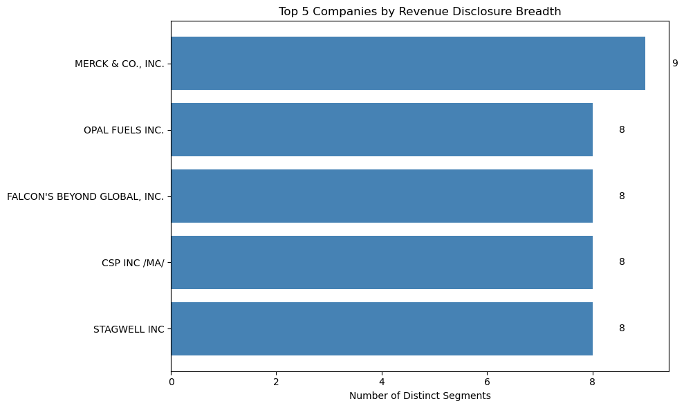
Disclosures segmented by Business Unit
While companies file disclosures for the overall entity, some prefer to file disclosures for each operational segment individually. The query below extracts the number of disclosures by company and segment. Here, we only focus on companies that have more than one disclosure.
sql_query3 = ("""
            SELECT s.adsh,s.name,
            MAX(n.ddate) AS latest_due_date,
            s.filed,
            s.accepted, n.segments,t.tlabel, s.form,
            s.fp,
            count(s.adsh) as num_submissions
            FROM sub_data s
            JOIN num_data n
            ON s.adsh = n.adsh
            AND n.tag = 'Revenues'
            JOIN tag_data t
            ON t.tag = n.tag
            GROUP BY s.adsh, s.name,
            s.filed, s.accepted,
            n.segments,
            t.tlabel,
            s.form,
            s.fp
            HAVING count(s.adsh) > 1
            ORDER BY 10 DESC
            """)
#Setup the URL to be used to invoke the GridDB WebAPI to retrieve data from the container
url = base_url + 'sql'

# Construct the request body
request_body = json.dumps([
    {
        "type": "sql-select",
        "stmt": sql_query3
    }
])

# Disable HTTP debugging
http.client.HTTPConnection.debuglevel = 0

#Invoke the GridDB WebAPI
data_req3 = requests.post(url, data=request_body, headers=header_obj)

#Process the response received and construct a Pandas dataframe with the data from the response
myJson = data_req3.json()
submissions_count = pd.DataFrame(myJson[0]["results"], columns=[myJson[0]["columns"][0]["name"], myJson[0]["columns"][1]["name"], myJson[0]["columns"][2]["name"], myJson[0]["columns"][3]["name"], myJson[0]["columns"][4]["name"], myJson[0]["columns"][5]["name"],myJson[0]["columns"][6]["name"],myJson[0]["columns"][7]["name"],myJson[0]["columns"][8]["name"],myJson[0]["columns"][9]["name"]])
submissions_count.head(n=5)
| adsh | name | |
|---|---|---|
| 0 | 0001558370-25-006523 | EVGO INC. |
| 1 | 0001628280-25-024374 | RICHMOND MUTUAL BANCORPORATION, INC. |
| 2 | 0001628280-25-023818 | INGRAM MICRO HOLDING CORP |
| 3 | 0001437749-25-021440 | CHARLIE'S HOLDINGS, INC. |
| 4 | 0001750155-25-000031 | CHARLOTTE'S WEB HOLDINGS, INC. |
def extract_segment_keys(segment_str):
    if pd.isna(segment_str):
        return []
    return [pair.split('=')[0] for pair in segment_str.strip(';').split(';') if '=' in pair]

# Create a new column with list of keys
submissions_count['segment_keys'] = submissions_count['segments'].apply(extract_segment_keys)

# Explode the list into separate rows
exploded = submissions_count[['name', 'segment_keys']].explode('segment_keys')

# Drop NaNs and count unique keys per company
segment_summary = (
    exploded.dropna()
    .groupby('name')['segment_keys']
    .nunique()
    .reset_index(name='distinct_segments')
    .sort_values(by='distinct_segments', ascending=False)
)
# Plot setup
plt.figure(figsize=(10, 6))
bars = plt.barh(top5['name'], top5['distinct_segments'], color='steelblue')

# Axis labels and title
plt.xlabel('Number of Distinct Segments')
plt.title('Top 5 Companies by Revenue Disclosure Breadth')
plt.gca().invert_yaxis()  # Highest at the top

# Annotate each bar with its value
for bar in bars:
    width = bar.get_width()
    plt.text(width + 0.5, bar.get_y() + bar.get_height()/2,
             f'{int(width)}', va='center', fontsize=10)

plt.tight_layout()
plt.show()

Insight(s): Merck & Co, Inc., Opal Fuels Inc, Falcon's, CSP, and Stagwell submit multiple revenue disclosures by segment, exhibiting greater financial transparency, and also suggest that these companies operate across multiple disciplines.
Million Dollar Companies that operated at a loss as of 2025 Q2
Here, we are interested in identifying companies that reported exceptionally high revenue (greater than USD 100 million) while simultaneously submitting a significant net loss of negative USD 500 million in their disclosures. The results can be further used to understand why such companies end up incurring a loss despite earning an exceedingly high revenue. Moreover, this contrast highlights entities that may have too many operating and administrative expenses or supply chain fluctuations that corrode the revenue. In this case, we use GridDB's intersect operation. Refer to this resource to learn more.
sql_query4 = ("""
            SELECT a.adsh, a.name
            FROM (
                SELECT s.adsh, s.name, SUM(n.value) revenue
                FROM sub_data s
                JOIN num_data n ON s.adsh = n.adsh
                WHERE n.tag IN ('Revenues')
                AND n.uom = 'USD'
                GROUP BY s.adsh, s.name
            ) a
            WHERE a.revenue > 100000000
            INTERSECT
            SELECT b.adsh, b.name
            FROM (
                SELECT s.adsh, s.name, sum(n.value) netincomeloss
                FROM sub_data s
                JOIN num_data n ON s.adsh = n.adsh
                WHERE n.tag = 'NetIncomeLoss'
                AND n.uom = 'USD'
                GROUP BY s.adsh, s.name
            ) b
            WHERE b.netincomeloss < -500000000

            """)
#Setup the URL to be used to invoke the GridDB WebAPI to retrieve data from the container
url = base_url + 'sql'

# Construct the request body
request_body = json.dumps([
    {
        "type": "sql-select",
        "stmt": sql_query4
    }
])

# Disable HTTP debugging
http.client.HTTPConnection.debuglevel = 0

#Invoke the GridDB WebAPI
data_req4 = requests.post(url, data=request_body, headers=header_obj)

#Process the response received and construct a Pandas dataframe with the data from the response
myJson = data_req4.json()
R_D_Companies_count = pd.DataFrame(myJson[0]["results"], columns=[myJson[0]["columns"][0]["name"], myJson[0]["columns"][1]["name"]])
# Create Plotly Table
fig = go.Figure(data=[go.Table(
    header=dict(
        values=list(R_D_Companies_count.columns),
        fill_color='lightblue',
        align='left',
        font=dict(color='black', size=12)
    ),
    cells=dict(
        values=[R_D_Companies_count[col] for col in R_D_Companies_count.columns],
        fill_color='white',
        align='left',
        font=dict(color='black', size=11)
    )
)])

fig.update_layout(
    title='Million-Dollar Companies That Operated at a Loss (2025 Q2)'
)

fig.show()
Insight(s): Affirm Holdings Inc., Medical Properties Trust Inc., among others, reported a net loss despite generating a revenue of more than $100M as of 2025 Q2.
Density Distribution of Companies based on Profit-Loss Status
With the below query, we gather the number of companies and their average net income by geography. We use a combination of subqueries, joins, and unions in this case.
sql_query5 = ("""SELECT
                cityba,
                stprba,
                countryba,
                status,
                COUNT(DISTINCT name) AS company_count,
                AVG(netincomeloss) AS avg_net_income
                FROM (
                    SELECT s.adsh, s.name, s.cityba,
                    s.stprba, s.countryba,
                    n.value AS netincomeloss,
                    'Profit' AS status
                    FROM sub_data s
                    JOIN num_data n ON s.adsh = n.adsh
                    WHERE n.tag = 'NetIncomeLoss' AND n.value > 0
                    UNION
                    SELECT s.adsh, s.name, s.cityba,
                    s.stprba, s.countryba,
                    n.value AS netincomeloss,
                    'Loss' AS status
                    FROM sub_data s
                    JOIN num_data n ON s.adsh = n.adsh
                    WHERE n.tag = 'NetIncomeLoss' AND n.value < 0
                    ) AS profit_loss
                GROUP BY cityba, stprba, countryba, status;
""")
#Setup the URL to be used to invoke the GridDB WebAPI to retrieve data from the container
url = base_url + 'sql'

# Construct the request body
request_body = json.dumps([
    {
        "type": "sql-select",
        "stmt": sql_query5
    }
])

# Disable HTTP debugging
http.client.HTTPConnection.debuglevel = 0

#Invoke the GridDB WebAPI
data_req5 = requests.post(url, data=request_body, headers=header_obj)

#Process the response received and construct a Pandas dataframe with the data from the response
myJson = data_req5.json()
density_distribution = pd.DataFrame(myJson[0]["results"], columns=[myJson[0]["columns"][0]["name"], myJson[0]["columns"][1]["name"],myJson[0]["columns"][2]["name"],myJson[0]["columns"][3]["name"],myJson[0]["columns"][4]["name"],myJson[0]["columns"][5]["name"]])
density_distribution['log_income'] = density_distribution['avg_net_income'].apply(
    lambda x: np.sign(x) * np.log1p(abs(x))
)
# Convert ISO-2 to ISO-3
def iso2_to_iso3(code):
    try:
        return pycountry.countries.get(alpha_2=code).alpha_3
    except:
        return None

density_distribution['iso3'] = density_distribution['countryba'].apply(iso2_to_iso3)


fig = px.choropleth(
    density_distribution,
    locations='iso3',               # ISO 2-letter codes like 'US', 'CN'
    locationmode='ISO-3',
    color='log_income',
    hover_name='countryba',
    hover_data=['company_count', 'avg_net_income'],
    color_continuous_scale='RdYlGn',
    title='Average Net Income by Country'
)

fig.data[0].zmid = 0

fig.update_layout(margin={"r":0,"t":40,"l":0,"b":0})
fig.show()
Insight(s): - United States, China, India, Germany, and the United Kingdom are the green zones representing high profitability. Brazil, Australia, South Africa, Mexico, several Southeast Asian and Latin American countries represent the net loss territories. Canada, France, Japan, South Korea, Spain represent the orange zones with mixed profitability.
Concluding Remarks
In this article, we saw how GridDB helped with a structured analysis of SEC filings. We were able to dissect data by effectively combining multiple containers to align financial metrics with the associated metadata tags. While we got rich insights on the SEC financial dataset, we were also able to explore GridDB's schema flexibility, wherein schemas could be created and modified programmatically using the API. We also learned how GridDB's NewSQL Interface and its ability to treat containers like tables could help onboard existing relational database developers onto GridDB easily.
If you have any questions about the blog, please create a Stack Overflow post here https://stackoverflow.com/questions/ask?tags=griddb .
Make sure that you use the “griddb” tag so our engineers can quickly reply to your questions.