
Customer churn is a key business concept that determines the number of customers that stop doing business with a specific company. The churn rate is then defined as the rate by which a company loses customers in a given time frame. For example, a churn rate of 15%/year means that a company loses 15% of its total customer base every year. Customer churn takes special importance in the telecommunication sector, given the increasing competition and appearance of new telecommunication companies. For this reason, the telecom industry expects high churn rates every year.
The churn rate in the telecom industry is approximately 1.9% every month and can raise to 67% every year. Source
This directly impacts the customer retention rate, a risk that companies consider very carefully.
As explained by the same article, the cost of acquisition of new customers in the telecom industry is 25 times greater that the cost of customer retention; another reason that makes churn rate decisive in this sector.
Advanced machine learning algorithms collaborate with business concepts like retention rate to provide business intelligence solutions. In this article, we describe a model to predict the churn rate in the telecom industry thanks to an extensive and detailed dataset. For this purpose we combine a set of technologies including Python, GridDB and machine learning algorithms, to deploy this solution in a real-life production environment. In this article, we begin by setting up the execution of environment. Then we introduce the dataset used in this study. We also import the necessary Python libraries to load the dataset. We make use of different python libraries to explore the dataset. After that, we describe the model of the machine learning algorithm that we evaluate to obtain the prediction results.
Setting up your environment
In order to successfully complete the operations performed in this article, here is a list of things to recreate our context of executions:
- Windows 10, Anaconda, Jupiter Notebook
- Python 3.8 – MSI for GridDB Python Client 0.8.3
- MSI for GridDB C Client –
- Swig 4.0.2
For GridDB Python client installation using pip, please refer to the following links: pip install griddb-python-client pip install griddb-python
Introduction to the dataset
The dataset used in this article is representative as it counts with 7043 rows each representing a customer. The dataset has 27 different attributes. The dataset is open source and is available in the following Kaggle notebook. Here are some of the important attributes that will be mentioned later in the article:
Gender: customer is male or femaleSeniorCitizen: customer is senior citizen of norTenure: number of months of customer business with the companyOnlineSecurity: customer has online security or not- Other attributes like
PhoneService,MultipleLines,InternetService
We will further investigate the attributes as well as their types in future sections.
Importing the necessary libraries
In other to accomplish the process explained in this article, we will need to import some Python libraries. In our Jupyter notebook, we insert the following lines:
import numpy as nump # linear algebra
import pandas as pand #  data processing, read CSV file
import seaborn as seab#  data visualization
import matplotlib.pyplot as plot #calculate plots
import griddb_python as griddb #application database
Loading the Dataset
In order to load the dataset we make use of the pandas library that we imported in the previous section:
telecom_customers = pand.read_csv('Churn.csv')We use pandas library to get an extract of the dataset, thanks to the head function, that looks as follows:
telecom_customers.head()customerID gender SeniorCitizen Partner Dependents tenure PhoneService MultipleLines InternetService OnlineSecurity ... DeviceProtection TechSupport StreamingTV StreamingMovies Contract PaperlessBilling PaymentMethod MonthlyCharges TotalCharges Churn
0 7590-VHVEG Female 0 Yes No 1 No No phone service DSL No ... No No No No Month-to-month Yes Electronic check 29.85 29.85 No
1 5575-GNVDE Male 0 No No 34 Yes No DSL Yes ... Yes No No No One year No Mailed check 56.95 1889.5 No
2 3668-QPYBK Male 0 No No 2 Yes No DSL Yes In order to build our GridDB database model, we need to obtain all the attributes of the database. For this we use the following line:
telecom_customers.columns.valuesThis command outputs an array containing all attribute names:
array(['customerID', 'gender', 'SeniorCitizen', 'Partner', 'Dependents',
       'tenure', 'PhoneService', 'MultipleLines', 'InternetService',
       'OnlineSecurity', 'OnlineBackup', 'DeviceProtection',
       'TechSupport', 'StreamingTV', 'StreamingMovies', 'Contract',
       'PaperlessBilling', 'PaymentMethod', 'MonthlyCharges',
       'TotalCharges', 'Churn'], dtype=object)
However, we need to know the data types of these attributes in order to map them with the GridDB database model. For this purpose, we use the following line:
Telecom_customers.dtypesAnd we obtain the types of all attributes:
customerID           object
gender               object
SeniorCitizen         int64
Partner              object
Dependents           object
tenure                int64
PhoneService         object
MultipleLines        object
InternetService      object
OnlineSecurity       object
OnlineBackup         object
DeviceProtection     object
TechSupport          object
StreamingTV          object
StreamingMovies      object
Contract             object
PaperlessBilling     object
PaymentMethod        object
MonthlyCharges      float64
TotalCharges         object
Churn                object
dtype: objec
First, we will begin by detecting the null values in our dataset and replacing them with any value. We will also remove the customerID column, as it is not relevant for our data model. We will also replace the churn attribute values from Yes/No to a boolean True/False to match our GridDB data architecture. In fact, as we will define most attributes as booleans, we will do this with all categorical attributes of the dataset. This is achieved with the following lines of code:
telecom_customers.dropna(inplace = True)

dataframe = telecom_customers.iloc[:,1:]

dataframe['Churn'].replace(to_replace='Yes', value=True, inplace=True)
dataframe['Churn'].replace(to_replace='No',  value=False, inplace=True)
Also, we will replace all categorical attributes into dummy variables. We will see in later sections that these dummy variables will be used to build our machine learning algorithm:
dataframeDummies = pand.get_dummies(dataframe)
dataframeDummies.head()
As we can observe, boolean attributes like gender, are now treated as booleans, instead of objects. Having this in mind, we begin building our GridDB database mode, by mapping each of the attributes of the dataset to GridDB:
conInfo = griddb.ContainerInfo("column1",
                    [["customerID", griddb.Type.STRING],
                    ["gender", griddb.Type.STRING],
                    ["SeniorCitizen", griddb.Type.BOOL],
                    ["Partner", griddb.Type.BOOL],
                    ["Dependents", griddb.Type.BOOL],
                    ["tenure", griddb.Type.LONG],
                    ["PhoneService", griddb.Type.BOOL],
                    ["MultipleLines", griddb.Type.BOOL],
                    ["InternetService", griddb.Type.STRING],
                    ["OnlineSecurity", griddb.Type.BOOL],
                    ["OnlineBackup", griddb.Type.BOOL],
                    ["DeviceProtection", griddb.Type.BOOL],
                    ["TechSupport", griddb.Type.BOOL],
                    ["StreamingTV", griddb.Type.BOOL],
                    ["StreamingMovies", griddb.Type.BOOL],
                    ["Contract", griddb.Type.String],
                    ["PaperlessBilling", griddb.Type.BOOL],
                    ["PaymentMethod", griddb.Type.STRING],
                    ["MonthlyCharges", griddb.Type.FLOAT],
                    ["TotalCharges", griddb.Type.FLOAT],
                    ["Churn", griddb.Type.BLOB]],
                    griddb.ContainerType.COLLECTION, True)
    col = gridstore.put_container(conInfo)
For more information on how to obtain a GridDB instance, a store, and create a collection, please visit the official GitHub repository, which includes multiple samples for GridDB in Python.
Do not forget to add an index for the primary key of the model, the customerID:
col.create_index("customerID", griddb.IndexType.DEFAULT)
Now we need to obtain the data in the dataset and store it in GridDB. We achieve this with the following code:
filename = 'churn.csv'
    with open(filename, 'r') as csvfile:
    datareader = csv.reader(csvfile)
    for row in datareader:
        toGriddb = col.put(row)
    col.commit();
To make sure that the data was uploaded correctly, we perform a query:
query=col.query("select * where gender = 'Female'")After we have verified that GridDB successfully holds the data, let us continue by an exploratory data analysis.
Exploratory Data Analysis
At this point, we are ready to perform an exploratory data analysis. First, we should begin by establishing a correlation between the attributes in the dataset with the churn attribute, the main focus of our study. To perform this correlation, we use the following line of code:
plot.figure(figsize=(15,8))
dataframe_dummies.corr()['Churn'].sort_values(ascending = False).plot(kind='bar')
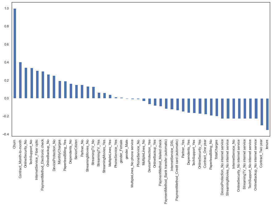
Let us analyze the results of this correlation graph. From right to left, we observe churn attribute, that as expected, has a correlation of 1 with itself. Other attributes that have a high correlation with churn are contracts, online security, and technical support. In another hand, from left to right, two-year contracts and tenure, as the customers are retained, have a negative correlation with churn.
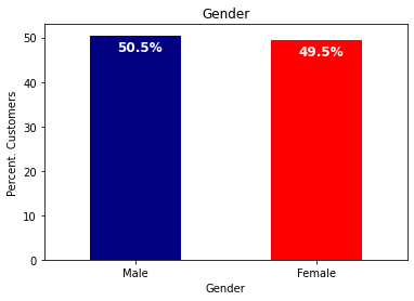
Now, depending on the interest of our study, we can plot various variables in our dataset, using the matplotlib.ticker library. For demonstration purposes, we would like to plot the gender variable in our dataset and see the percentage of men and women customers. This is achieved with the following code:
colors = ['#000080','#FF0000']
ax = (telecom_customers['gender'].value_counts()*100.0 /len(telecom_customers)).plot(kind='bar',stacked = True,rot = 0,color = colors)

ax.set_ylabel('Percent. Customers')
ax.set_xlabel('Gender')
ax.set_ylabel('Percent. Customers')
ax.set_title('Gender')

totals = []

for i in ax.patches:
    totals.append(i.get_width())

total = sum(totals)

for i in ax.patches:
    ax.text(i.get_x()+.15, i.get_height()-3.5,
            str(round((i.get_height()/total), 1))+'%',
            fontsize=12,
            color='white',
           weight = 'bold')
And outputs the following graph:
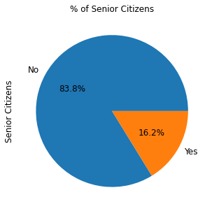
Let us take another example, and plot our customers by senior citizenship, using the a similar code:
ax = (telecom_customers['SeniorCitizen'].value_counts()*100.0 /len(telecom_customers))
.plot.pie(autopct='%.1f%%', labels = ['No', 'Yes'],figsize =(5,5), fontsize = 12 )

ax.set_ylabel('Senior Citizens',fontsize = 12)
ax.set_title('% of Senior Citizens', fontsize = 12)
To obtain the following pie chart:
Now we have our data ready, it is time to predict the churn of customers. In the next section, we describe the machine learning model used in this article to predict the churn rate.
Machine Learning Model
Before building the model, we must recall that we have already transformed all categorical variables into dummy attributes. This process will make the implementation of machine learning easier for all the attributes of the dataset, and we will not have to use multiple functions. In fact, we will be using this dummy data frame that we created in earlier sections, and we will also scale the variables to a value between 0 and 1, to be more suitable for the algorithm. These two operations are achieved with the following code:
y = dataframe_dummies['Churn'].values
X = dataframe_dummies.drop(columns = ['Churn'])

from sklearn.preprocessing import MinMaxScaler
features = X.columns.values
scaler = MinMaxScaler(feature_range = (0,1))
scaler.fit(X)
X = pand.DataFrame(scaler.transform(X))
X.columns = features
In order to use the machine learning algorithm, we will have to randomly split the dataset to provide both the training and the testing data. This is achieved with the following lines of code:
from sklearn.model_selection import train_test_split
X_train, X_test, y_train, y_test = train_test_split(X, y, test_size=0.3, random_state=101)
For the purpose of this study, we will use a logistic regression model to predict the churn rate. We will begin by fitting the regression model to our training data.
from sklearn.linear_model import LogisticRegression
model = LogisticRegression()
result = model.fit(X_train, y_train)
Model Evaluation
At this moment, we are ready to run the model. To do that, we use the predict() function from the LogisticRegression library to make a prediction on the actual testing data. We can observe that the obtained accuracy is 80% of correctly classified instances.
from sklearn import metrics
from sklearn.metrics import classification_report, confusion_matrix

prediction_test = model.predict(X_test)

# Print results & confusion matrix
print (metrics.accuracy_score(y_test, prediction_test))

print(confusion_matrix(y_test,prediction_test))
0.8075829383886256
Now, we will see how to interpret the confusion matrix:
[1418  162]
[ 244  286]
We can observe from the results that 1418 and 286 were respectively the true positives and false positives, or the correctly classified instances, in this case, the likelihood of a customer to churn. The sum of these instances is 1704, which represents 80% of the total 2110 instances.
Conclusion
In this article, we have seen predicted churn in the telecommunication industry using machine learning algorithms in Python. As a database to store our data, we used GridDB.
In case you would like to take this article a step further, you can try with other classification algorithms that can be executed in a similar way to the example provided in this article. For more details, visit the open source notebook.
References
- https://www.heavy.ai/blog/strategies-for-reducing-churn-rate-in-the-telecom-industry
- https://www.kaggle.com/bandiatindra/telecom-churn-prediction/notebook