
In this tutorial, we will see how to analyze time-series data stored in GridDB using Python. The outline of the tutorial is as follows –
- Loading the dataset using SQL and Pandas
- Preprocess the data to deal with null, missing values, etc.
- Build a classifier for our data
Prerequisites
This tutorial assumes prior installation of GridDB, Python3, and the associated libraries. If you have not installed any of the below packages, go ahead and do it before continuing with the tutorial. 1. GridDB 2. Python 3 3. GridDB Python Client 4. NumPy 5. Pandas 6. Matplotlib 7. Scikit-learn 8. Lightgbm 9. Seaborn
The following tutorial is carried out in Jupyter notebooks (Anaconda Navigator). You can install these packages directly in your environment using conda install package_name. Alternatively, type pip install package_name in the command prompt/terminal.
Importing the necessary libraries
Once you are done installing the required packages, let’s import these libraries.
import numpy as np
import pandas as pd
import matplotlib.pyplot as plt
from sklearn.preprocessing import *
from sklearn.model_selection import *
from sklearn.metrics import *
import os
from datetime import datetime
import time
from lightgbm import LGBMRegressor
import seaborn as sns
from sklearn import metrics
APP_PATH = os.getcwd()
APP_PATH'C:\Users\SHRIPRIYA\Desktop\AW Group\GridDB'
Loading the dataset
The time-series dataset we’re using for this tutorial has been open-sourced on Kaggle. The zip folder contains two separate files for training and testing. However, since the test dataset does not contain the labels, we will not be able to verify our model’s performance. Therefore, will be using the training file as the whole dataset, and later on, we will split it into Train and Test sets.
The training file has about 48000 rows (or instances) with 4 columns (or attributes) – ID, DateTime, Junction, and Vehicles. Column Vehicle is the dependent (or response) variable while DateTime and Junction are independent (or explanatory) variables
Using SQL
You can type the following statement in your Python script or console to retrieve the data from GridDB. The advantage of using GridDB’s python-client is that the resulting data type is a pandas dataframe. This makes data manipulation much easier.
statement = ('SELECT * FROM train_ml_iot')

dataset = pd.read_sql_query(statement, cont)
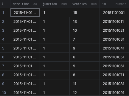
The output will look like –
Getting to know the dataset
Now that we have loaded our dataset, it is time to get a peek at how it looks. We can print out the first 5 rows using the head command. If you want to print more rows, simply pass a number to the function as an argument. For instance, dataset.head(15) will print out the first 15 rows. You can also use the tail command to get a gist of the dataset. The only difference is, as the name suggests, it prints the last 5 rows.
dataset.head()| DateTime | Junction | Vehicles | ID | |
|---|---|---|---|---|
| 0 | 2015-11-01 00:00:00 | 1 | 15 | 20151101001 |
| 1 | 2015-11-01 01:00:00 | 1 | 13 | 20151101011 |
| 2 | 2015-11-01 02:00:00 | 1 | 10 | 20151101021 |
| 3 | 2015-11-01 03:00:00 | 1 | 7 | 20151101031 |
| 4 | 2015-11-01 04:00:00 | 1 | 9 | 20151101041 |
len(dataset)48120
describe() command is useful when dealing with numerical data. It basically prints out the whole summary of your data such as min, max, average, etc. We can use this information to know the range and scale of each attribute. There does not seem any anomaly from this level. Also, the scale of the attributes is not that different. This means we can skip the feature scaling step for this dataset.
dataset.describe()| Junction | Vehicles | ID | |
|---|---|---|---|
| count | 48120.000000 | 48120.000000 | 4.812000e+04 |
| mean | 2.180549 | 22.791334 | 2.016330e+10 |
| std | 0.966955 | 20.750063 | 5.944854e+06 |
| min | 1.000000 | 1.000000 | 2.015110e+10 |
| 25% | 1.000000 | 9.000000 | 2.016042e+10 |
| 50% | 2.000000 | 15.000000 | 2.016093e+10 |
| 75% | 3.000000 | 29.000000 | 2.017023e+10 |
| max | 4.000000 | 180.000000 | 2.017063e+10 |
Data Preprocessing
As mentioned above, the two attributes – DateTime and Junction are the independent variables and therefore, contribute to the outcome variable i.e.Vehicles. Therefore, keeping the ID attribute seems unnecessary. Let’s go ahead and drop it.
dataset.drop(["ID"],axis = 1,inplace=True)Nobody likes redundant data. Let’s drop that too!
dataset.drop_duplicates(keep="first", inplace=True)
len(dataset)
48120
Fortunately, the dataset did not have any duplicates, but it’s always a good practice to check for redundancy. Dealing with null values is also important when dealing with numerical data, especially. Null values make it difficult to perform mathematical operations and can also result in errors. So, you either replace null values with dummy data or drop those rows. Let’s first check if our data contains any null values.
dataset.isnull().sum()DateTime 0
Junction 0
Vehicles 0
dtype: int64
dataset.dtypesDateTime object
Junction int64
Vehicles int64
dtype: object
The DateTime attribute has the datatype object. We will first call the pandas function to_datetime to convert this attribute to its actual format. This will allow us to extract the information about the year, month, day, etc, directly.
dataset['DateTime'] = pd.to_datetime(dataset['DateTime'])Great! Now that our time is converted to a suitable format, let’s extract the following attributes – Weekday, Year, Month, Day, Time, Week, and Quater
dataset['Weekday'] = [date.weekday() for date in dataset.DateTime]
dataset['Year'] = [date.year for date in dataset.DateTime]
dataset['Month'] = [date.month for date in dataset.DateTime]
dataset['Day'] = [date.day for date in dataset.DateTime]
dataset['Time'] = [((date.hour*60+(date.minute))*60)+date.second for date in dataset.DateTime]
dataset['Week'] = [date.week for date in dataset.DateTime]
dataset['Quarter'] = [date.quarter for date in dataset.DateTime]
The updated dataset looks like –
dataset.head()| DateTime | Junction | Vehicles | Weekday | Year | Month | Day | Time | Week | Quarter | |
|---|---|---|---|---|---|---|---|---|---|---|
| 0 | 2015-11-01 00:00:00 | 1 | 15 | 6 | 2015 | 11 | 1 | 0 | 44 | 4 |
| 1 | 2015-11-01 01:00:00 | 1 | 13 | 6 | 2015 | 11 | 1 | 3600 | 44 | 4 |
| 2 | 2015-11-01 02:00:00 | 1 | 10 | 6 | 2015 | 11 | 1 | 7200 | 44 | 4 |
| 3 | 2015-11-01 03:00:00 | 1 | 7 | 6 | 2015 | 11 | 1 | 10800 | 44 | 4 |
| 4 | 2015-11-01 04:00:00 | 1 | 9 | 6 | 2015 | 11 | 1 | 14400 | 44 | 4 |
dataset.keys()Index(['DateTime', 'Junction', 'Vehicles', 'Weekday', 'Year', 'Month', 'Day',
'Time', 'Week', 'Quarter'],
dtype='object')
Visualizing the trend
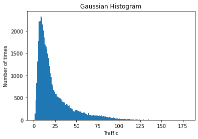
Let’s see if there are any patterns our data is following.
data = dataset.Vehicles
binwidth = 1
plt.hist(data, bins=range(min(data), max(data) + binwidth, binwidth), log=False)
plt.title("Gaussian Histogram")
plt.xlabel("Traffic")
plt.ylabel("Number of times")
plt.show()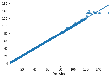
We can see that, more often than not, the traffic lies between (20,30) given a certain timestamp. That’s not too bad.
Preparing the dataset for Model Building
The datetounix function converts the DateTime attribute to unixtime. A unix timestamp is simply a number denoting the total time elapsed (in seconds) since the Unix Epoch. As its definition suggests, a unix timestamp is timezone independent which is why it is frequently used during Model Building.
def datetounix(df):
    unixtime = []

    # Running a loop for converting Date to seconds
    for date in df['DateTime']:
        unixtime.append(time.mktime(date.timetuple()))

    # Replacing Date with unixtime list
    df['DateTime'] = unixtime
    return(df)
dataset_features = datetounix(dataset)dataset_features| DateTime | Junction | Vehicles | Weekday | Year | Month | Day | Time | Week | Quarter | |
|---|---|---|---|---|---|---|---|---|---|---|
| 0 | 1.446316e+09 | 1 | 15 | 6 | 2015 | 11 | 1 | 0 | 44 | 4 |
| 1 | 1.446320e+09 | 1 | 13 | 6 | 2015 | 11 | 1 | 3600 | 44 | 4 |
| 2 | 1.446323e+09 | 1 | 10 | 6 | 2015 | 11 | 1 | 7200 | 44 | 4 |
| 3 | 1.446327e+09 | 1 | 7 | 6 | 2015 | 11 | 1 | 10800 | 44 | 4 |
| 4 | 1.446331e+09 | 1 | 9 | 6 | 2015 | 11 | 1 | 14400 | 44 | 4 |
| … | … | … | … | … | … | … | … | … | … | … |
| 48115 | 1.498829e+09 | 4 | 11 | 4 | 2017 | 6 | 30 | 68400 | 26 | 2 |
| 48116 | 1.498833e+09 | 4 | 30 | 4 | 2017 | 6 | 30 | 72000 | 26 | 2 |
| 48117 | 1.498837e+09 | 4 | 16 | 4 | 2017 | 6 | 30 | 75600 | 26 | 2 |
| 48118 | 1.498840e+09 | 4 | 22 | 4 | 2017 | 6 | 30 | 79200 | 26 | 2 |
| 48119 | 1.498844e+09 | 4 | 12 | 4 | 2017 | 6 | 30 | 82800 | 26 | 2 |
48120 rows × 10 columns
X = dataset_features Junction, Weekday, and Day are discrete data – they are classes rather than a continuous value. Therefore, we need to encode this data before passing it to the classifier. For that, these data will need to be converted to str. Then, we will call the get_dummies function to get the encoded data.
X['Junction'] = X['Junction'].astype('str')
X['Weekday']  = X['Weekday'].astype('str')
X['Day'] = X[ 'Day' ].astype('str')
X = pd.get_dummies(X)print("X.shape : ", X.shape)
display(X.columns)X.shape : (48120, 49)
Index(['DateTime', 'Vehicles', 'Year', 'Month', 'Time', 'Week', 'Quarter',
'Junction_1', 'Junction_2', 'Junction_3', 'Junction_4', 'Weekday_0',
'Weekday_1', 'Weekday_2', 'Weekday_3', 'Weekday_4', 'Weekday_5',
'Weekday_6', 'Day_1', 'Day_10', 'Day_11', 'Day_12', 'Day_13', 'Day_14',
'Day_15', 'Day_16', 'Day_17', 'Day_18', 'Day_19', 'Day_2', 'Day_20',
'Day_21', 'Day_22', 'Day_23', 'Day_24', 'Day_25', 'Day_26', 'Day_27',
'Day_28', 'Day_29', 'Day_3', 'Day_30', 'Day_31', 'Day_4', 'Day_5',
'Day_6', 'Day_7', 'Day_8', 'Day_9'],
dtype='object')
X.head()| DateTime | Vehicles | Year | Month | Time | Week | Quarter | Junction_1 | Junction_2 | Junction_3 | … | Day_29 | Day_3 | Day_30 | Day_31 | Day_4 | Day_5 | Day_6 | Day_7 | Day_8 | Day_9 | |
|---|---|---|---|---|---|---|---|---|---|---|---|---|---|---|---|---|---|---|---|---|---|
| 0 | 1.446316e+09 | 15 | 2015 | 11 | 0 | 44 | 4 | 1 | 0 | 0 | … | 0 | 0 | 0 | 0 | 0 | 0 | 0 | 0 | 0 | 0 |
| 1 | 1.446320e+09 | 13 | 2015 | 11 | 3600 | 44 | 4 | 1 | 0 | 0 | … | 0 | 0 | 0 | 0 | 0 | 0 | 0 | 0 | 0 | 0 |
| 2 | 1.446323e+09 | 10 | 2015 | 11 | 7200 | 44 | 4 | 1 | 0 | 0 | … | 0 | 0 | 0 | 0 | 0 | 0 | 0 | 0 | 0 | 0 |
| 3 | 1.446327e+09 | 7 | 2015 | 11 | 10800 | 44 | 4 | 1 | 0 | 0 | … | 0 | 0 | 0 | 0 | 0 | 0 | 0 | 0 | 0 | 0 |
| 4 | 1.446331e+09 | 9 | 2015 | 11 | 14400 | 44 | 4 | 1 | 0 | 0 | … | 0 | 0 | 0 | 0 | 0 | 0 | 0 | 0 | 0 | 0 |
5 rows × 49 columns
Defining a classifier
We will be using a gradient boosting model – LGBMRegressor. More information on the model architecture and parameters can be found here.
clf = LGBMRegressor(boosting_type='gbdt',
                    max_depth=6,
                    learning_rate=0.25,
                    n_estimators=80,
                    min_split_gain=0.7,
                    reg_alpha=0.00001,
                    random_state = 16
                   )
Splitting the dataset
Splitting the dataset into train and test with a ratio of 70-30. You can customize this ratio as per your convenience. We have used the conventional one.
Y = dataset['Vehicles'].to_frame()
dataset = dataset.drop(['Vehicles'], axis=1)
X_train, X_test, y_train, y_test = train_test_split(X, Y, test_size=0.3, random_state=101)
Model Evaluation
Let’s see how our model performs on the test data.
clf = clf.fit(X_train, y_train)predictions = clf.predict(X_test)print("RMSE", np.sqrt(metrics.mean_squared_error(y_test, predictions)))RMSE 0.309624242642493
sns.regplot(y_test,predictions)<matplotlib.axes._subplots.AxesSubplot at 0x138722cdcd0>
Conclusion
The model resulted in an RMSE of 0.309 which is pretty decent. You could try experimenting with different evaluation metrics. The resulting line in the plot seems to fit the data instances accurately. Thus, we could be assured that the model is performing well.
More information on Metrics and Scoring is available on the official website of scikit-learn. Happy Coding!