In this article, we will use GridDB to analyse how scientists decide whether or not asteroids are dangerous to Earth, that is, whether or not they will leave their orbit and land here on Earth, potentially harming the population.
Full source code can be found here: https://github.com/griddbnet/Blogs/tree/asteroids_distance
Exporting and Importing dataset using GridDB
GridDB is a highly scalable and optimized in-memory No SQL database that allows parallel processing for higher performance and efficiency, especially for time-series databases. We will be using GridDB’s node js client, which allows us to connect GridDB to node js and import or export data in real-time.
These are the columns that are present in our dataset:
- id : ID given to the asteroids by NASA scientists.
- new_name : Names given to the asteroids by NASA scientists.
- est_diameter_min : The minimum estimated diameter of the asteroids.
- est_diameter_max : The maximum estimated diameter of the asteroids.
- relative_velocity : The relative velocity of the asteroids compared to Earth.
- miss_distance : Asteroids’ distance away from the Earth.
- orbiting_body: Asteroids’ orbital around the specific body.
- sentry_object: Whether the asteroid collided with other body (satellites, etc) in the space.
- absolute_magnitude: The magnitude of force by which they would hit the Earth according to their mass-force ratio.
- hazardous : Are the asteroids at hazardous range? (Outcome Variable)
To upload the dataset to GridDB, we would read the CSV file that contains the data which is taken from This Kaggle Dataset
Now, we will create a GridDB container to pass our database schema to the GridDB to be able to generate the design of the database before inserting the row information. Next, we would insert our data into the GridDB. We have now successfully exported the dataset to the GridDB platform.
On the other hand, to import the dataset from the GridDB platform, we will use TQL, GridDB’s query language similar to SQL. We will create a container and store the fetched data in it. The next step would be to extract the rows in order of the column info and save it into a data frame to use for data visualization and analysis.
For the data visualization and analysis, we will be using the following library for NodeJS.
- DanfoJS – For working with DataFrames
var griddb = require('griddb_node');

const dfd = require("danfojs-node")
var fs     = require('fs');

const createCsvWriter = require('csv-writer').createObjectCsvWriter;
const csvWriter = createCsvWriter({
  path: 'out.csv',
  header: [
    {id: "id", title:"id"},
    {id: "new_name", title:"new_name"},
    {id: "est_diameter_min", title:"est_diameter_min"},
    {id: "est_diameter_max", title:"est_diameter_max"},
    {id: "relative_velocity", title:"relative_velocity"},
    {id: "miss_distance", title:"miss_distance"},
    {id: "orbiting_body" , title:"orbiting_body"},
    {id: "sentry_object", title:"sentry_object"},
    {id: "absolute_magnitude", title:"absolute_magnitude"}
  ]
});

const factory = griddb.StoreFactory.getInstance();
const store = factory.getStore({
    "host": '239.0.0.1',
    "port": 31999,
    "clusterName": "defaultCluster",
    "username": "admin",
    "password": "admin"
});

// For connecting to the GridDB Server we have to make containers and specify the schema.
const conInfo = new griddb.ContainerInfo({
    'name': "neoanalysis",
    'columnInfoList': [
      ["name", griddb.Type.STRING],
      ["id", griddb.Type.INTEGER],
        ["new_name", griddb.Type.STRING],
        ["est_diameter_min", griddb.Type.DOUBLE],
        ["est_diameter_max", griddb.Type.DOUBLE],
        ["relative_velocity", griddb.Type.DOUBLE],
        ["miss_distance", griddb.Type.DOUBLE],
        ["absolute_magnitude", griddb.Type.DOUBLE]
    ],
    'type': griddb.ContainerType.COLLECTION, 'rowKey': true
});


// ////////////////////////////////////////////


const csv = require('csv-parser');

const fs = require('fs');
var lst = []
var lst2 = []
var i =0;
fs.createReadStream('./Dataset/neo.csv')
  .pipe(csv())
  .on('data', (row) => {
    lst.push(row);
    console.log(lst);

  })
  .on('end', () => {
    var container;
    var idx = 0;

    for(let i=0;i<lst.length;i++){


    store.putContainer(conInfo, false)
        .then(cont => {
            container = cont;
            return container.createIndex({ 'columnName': 'name', 'indexType': griddb.IndexType.DEFAULT });
        })
        .then(() => {
            idx++;
            container.setAutoCommit(false);
            return container.put([String(idx), lst[i]['id'],lst[i]["new_name"],lst[i]["est_diameter_min"],lst[i]["est_diameter_max"],lst[i]["relative_velocity"],lst[i]["miss_distance"],lst[i]["absolute_magnitude"]]);
        })
        .then(() => {
            return container.commit();
        })

        .catch(err => {
            if (err.constructor.name == "GSException") {
                for (var i = 0; i < err.getErrorStackSize(); i++) {
                    console.log("[", i, "]");
                    console.log(err.getErrorCode(i));
                    console.log(err.getMessage(i));
                }
            } else {
                console.log(err);
            }
        });

    }
    store.getContainer("neoanalysis")
    .then(ts => {
        container = ts;
      query = container.query("select *")
      return query.fetch();
  })
  .then(rs => {
      while (rs.hasNext()) {


          let rsNext = rs.next()

          lst2.push(


            {
                'id': rsNext[1],
                "new_name": rsNext[2],
                "est_diameter_min": rsNext[3],
                "est_diameter_max": rsNext[4],
                "relative_velocity": rsNext[5],
                "miss_distance": rsNext[6],
                "absolute_magnitude": rsNext[7],

            }

          );

      }

        csvWriter
        .writeRecords(lst2)
        .then(()=> console.log('The CSV file was written successfully'));

      return
  }).catch(err => {
      if (err.constructor.name == "GSException") {
          for (var i = 0; i < err.getErrorStackSize(); i++) {
              console.log("[", i, "]");
              console.log(err.getErrorCode(i));
              console.log(err.getMessage(i));
          }
      } else {
          console.log(err);
      }
  });

  });
Data Analysis
We now check and load our dataset to conduct data analysis.
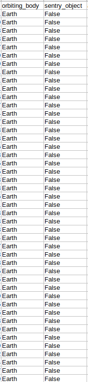
Because orbiting_body and sentry_object have redundant values throughout the column and no unique value to aid us in our analysis, we would omit these two columns from our analysis, as shown below.
We would load the csv file into the DataFrame variable(df) as shown below:
let df = await dfd.readCSV("./out.csv")Starting with our data analysis, we would first check the number of rows and columns in our dataset
We have 90836 rows and 8 columns.
console.log(df.shape)

//  Output
// [ 90836, 8 ]
Now to see the names of the columns after omitting two columns, as mentioned above, and the data types of the columns to get the idea of what the data represents:
console.log(df.columns)

// Output
// ['id','new_name', 'est_diameter_min', 'est_diameter_max', 'relative_velocity', 'miss_distance', 'absolute_magnitude', 'hazardous']
df.loc({columns:['id',
'new_name',
'est_diameter_min',
'est_diameter_max',
'relative_velocity',
'miss_distance','absolute_magnitude',
'hazardous']}).ctypes.print()
// Output
// ╔══════════════════════╤═════════╗
// ║ id │ int64 ║
// ╟──────────────────────┼─────────╢
// ║ new_name │ object ║
// ╟──────────────────────┼─────────╢
// ║ est_diameter_min │ float64 ║
// ╟──────────────────────┼─────────╢
// ║ est_diameter_max │ float64 ║
// ╟──────────────────────┼─────────╢
// ║ relative_velocity │ float64 ║
// ╟──────────────────────┼─────────╢
// ║ miss_distance │ float64 ║
// ╟──────────────────────┼─────────╢
// ║ absolute_magnitude │ float64 ║
// ╟──────────────────────┼─────────╢
// ║ hazardous │ bool ║
// ╚══════════════════════╧═════════╝We access the data from the GridDB container as follows:
    # Get the containers
    obtained_data = gridstore.get_container("redwinequality")

    # Fetch all rows - language_tag_container
    query = obtained_data.query("select *")
We will now look at a summary of statistics for the columns mentioned below to check their minimums, maximums, means, standard deviations etc.
df.loc({columns:['est_diameter_min','est_diameter_max','relative_velocity','miss_distance']}).describe().round(2).print()

// Output
// ╔════════════╤═══════════════════╤═══════════════════╤═══════════════════╤═══════════════════╗
// ║            │ est_diameter_min  │ est_diameter_max  │ relative_velocity │ miss_distance     ║
// ╟────────────┼───────────────────┼───────────────────┼───────────────────┼───────────────────╢
// ║ count      │ 90836             │ 90836             │ 90836             │ 9.1e+04           ║
// ╟────────────┼───────────────────┼───────────────────┼───────────────────┼───────────────────╢
// ║ mean       │ 0.13              │ 0.28              │ 48066             │ 3.71e+07          ║
// ╟────────────┼───────────────────┼───────────────────┼───────────────────┼───────────────────╢
// ║ std        │ 0.29              │ 0.67              │ 25293             │ 2.24e+07          ║
// ╟────────────┼───────────────────┼───────────────────┼───────────────────┼───────────────────╢
// ║ min        │ 0.00061           │ 0.0014            │ 203               │ 6.74e+03          ║
// ╟────────────┼───────────────────┼───────────────────┼───────────────────┼───────────────────╢
// ║ median     │ 0.05              │ 0.11              │ 44190             │ 3.78e+07          ║
// ╟────────────┼───────────────────┼───────────────────┼───────────────────┼───────────────────╢
// ║ max        │ 38                │ 85                │ 236990            │ 7.50e+07          ║
// ╟────────────┼───────────────────┼───────────────────┼───────────────────┼───────────────────╢
// ║ variance   │ 8.91e-02          │ 4.45e-01          │ 6.40e+08          │ 4.99e+14          ║
// ╚════════════╧═══════════════════╧═══════════════════╧═══════════════════╧═══════════════════╝
Now Plotting a Scatter Plot between Quality and the other Columns.
## Scatter Plot between miss_distance and relative_velocity
let cols = [...cols]
cols.pop('miss_distance')
for(let i = 0; i < cols.length; i++)
{
    let data = [{
        x: df[cols[i]].values,
        y: df['miss_distance'].values,
        type: 'scatter',
        mode: 'markers'}];
    let layout = {
        height: 400,
        width: 700,
        title: 'Missing Distance from Earth vs '+cols[i],
        xaxis: {title: cols[i]},
        yaxis: {title: 'Miss Distance'}};
    // There is no HTML element named `myDiv`, hence the plot is displayed below.
    Plotly.newPlot('myDiv', data, layout);
}
The plot for two example columns is below:
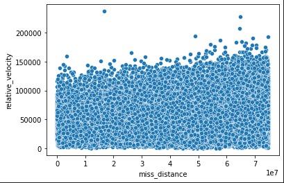
The plot above shows that the two variables have a positive linear relationship with other, which means that the greater missing distance from Earth, the greater the relative velocity since the asteroid would not be under the gravitational effect of Earth.
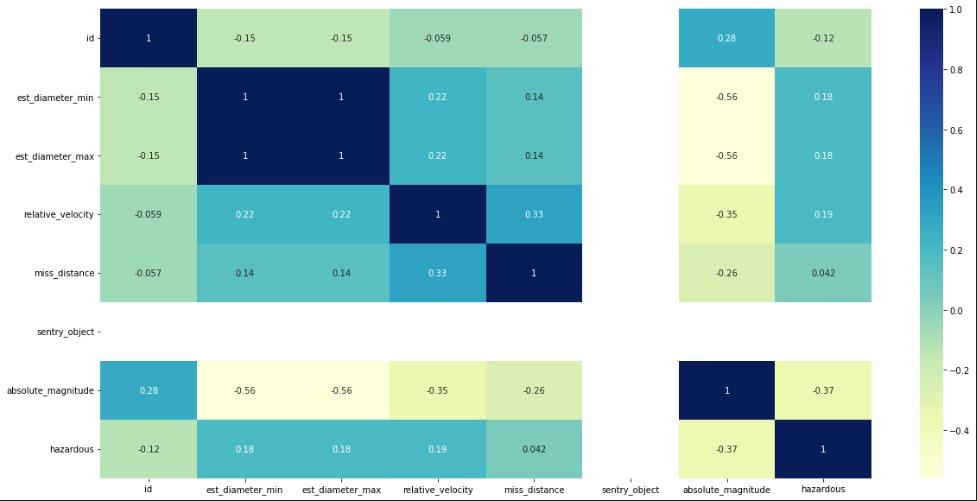
## Correlation plot of the columns to see how these variables or factors related to each other
correlogram(data)
The Correlation plot is below:

The correlation plot above shows the values for the variables, and the higher the value, the closer the relationships are between them. Thus, it is clear that miss distance and relative velocity have the highest values (0.33), indicating that they are the two most crucial variables in determining the point of impact for asteroid on Earth. The same variables will, however, naturally have the strongest correlations among themselves, so we disregard the diagonal above in the correlation plot.
Conclusion
NASA scientists consider a variety of variables when determining whether or not an asteroid will strike the Earth, and if it does, they need to know the precise coordinates in order to save as many precious human lives as possible.
Finally, all of this data analysis was done using GridDB because it facilitated quick access to and effective reading, writing, and storing of data.