
Introduction
Pandas Dataframes, as defined by their documentation, are data structures that are “Two-dimensional, size-mutable, potentially heterogeneous tabular data”. They essentially make performing data analysis quick and easy, allowing developers and data scientists to quickly perform experiments without having to write long blocks of code.
In this blog post we will demonstrate basic reading and writing between GridDB and a Pandas Dataframe, as well as some often-used transformations which GridDB developers may find useful.
Reading Data
To read data from GridDB into a data frame, you simply set up your query as normal and instead of a while rs.has_next() loop, you simply call rs.fetch_rows() which returns the DataFrame for that result set as demonstrated in the following example:
import datetime
import griddb_python as griddb
import sys
import pandas as pd
import matplotlib.pyplot as plt

factory = griddb.StoreFactory.get_instance()

argv = sys.argv

gridstore = factory.get_store(
    host="239.0.0.1",
    port=31999,
    cluster_name="defaultCluster",
    username="admin",
    password="admin"
)

col = gridstore.get_container("precinct_108")

start = datetime.datetime.utcnow().timestamp()
query = col.query("select *")
rs = query.fetch(False)
rows = rs.fetch_rows()
rows['CMPLNT_FR'] = pd.to_datetime(rows['CMPLNT_FR'])
print(rows)
Writing Data
Writing data to GridDB from a dataframe is also a simple operation. Create your ContainerInfo object that contains the data schema, open the container and call put_rows() with your dataframe as the argument. One word of caution, your schema column order and the dataframe column order must match but it is simple to re-order the dataframe by simply specifying the correct column order in a list in the specification.
conInfo = griddb.ContainerInfo("PANDAS_AGGS",
                [["key", griddb.Type.STRING],
                ["timestamp", griddb.Type.TIMESTAMP],
                ["precinct", griddb.Type.INTEGER],
                ["count", griddb.Type.INTEGER]],
            griddb.ContainerType.COLLECTION, True)

aggcn = gridstore.put_container(conInfo)
aggcn.put_rows(df[["key", "timestamp","precinct","count"]])
Simple Transformations
There are a many examples of simple operations you can performance with a Dataframe, but here are few:
Setting the value of a column:
df['precinct'] = 108
Combining two different columns, the same can be used for finding the sum or difference of each row.
df['key'] = df['CMPLNT_FR'].dt.strftime('%Y-%m-%d') +"_"+ df['precinct'].astype('str')
Renaming a column:
df = df.rename(columns={'CMPLNT_FR':'timestamp'})
Binning/Bucketing
In our Time Series Forecasting tutorial, we needed to transform individual complaints into the number of complaints reported per month. This required multiple nested for-loops. With Pandas Dataframes, we can accomplish the same thing with one line of code:
monthly_df = rows.groupby([pd.Grouper(key='CMPLNT_FR',freq='M')]).size().reset_index(name='count')
Now, at first glance the code is difficult to understand, the rows are split into groups defined by the input argument list, in this case every month that’s within the dataframe. The size of each of these groups is taken and put into the ‘count’ column.
It is often useful to also track event occurance by Day of the Week or Hour of the Day, in fact I often include a dayofweek and hourofday fields in schemas I build to easily query just data on Sundays or at 5pm. With a Pandas dataframe, both are just one liners.
weekly_df = rows.groupby(rows['CMPLNT_FR'].dt.day_name()).size().reset_index(name='count')
hourly_df  = rows.groupby(rows['CMPLNT_FR'].dt.hour).size().reset_index(name='count')
Performance
So what’s faster? Reading or writing to pyarrays or dataframes? What about binning?
Well, Pandas Dataframes have a downside, they’re slower.
We wrote a simple benchmark that writes and reads 10000 rows, writing a dataframe to GridDB is approximately 50% slower than multiputting the same data as a List of Lists.
blob = bytearray([65, 66, 67, 68, 69, 70, 71, 72, 73, 74])
conInfo = griddb.ContainerInfo("col01",
    [["name", griddb.Type.STRING],
    ["status", griddb.Type.BOOL],
    ["count", griddb.Type.LONG],
    ["lob", griddb.Type.BLOB]],
    griddb.ContainerType.COLLECTION, True)

i=0
rows=[]
while i < 10000:
    rows.append([str(uuid.uuid1()), False, random.randint(0, 1048576), blob])
    i=i+1

gridstore.drop_container("col01")
start =  datetime.datetime.utcnow().timestamp()
col = gridstore.put_container(conInfo)
col.multi_put(rows)
print("multiput took "+  str(datetime.datetime.utcnow().timestamp() - start) +" seconds")


df = pandas.DataFrame(rows, columns=["name", "status", "count", "lob"])

gridstore.drop_container("col01")
start =  datetime.datetime.utcnow().timestamp()
col = gridstore.put_container(conInfo)
col.put_rows(df)
col.multi_put(rows)
print("putrows took "+  str(datetime.datetime.utcnow().timestamp() - start) +" seconds")
Reading the data back found that appending the result set to a pylist was about 25% faster than reading it directly into a dataframe; reading the list and then converting to a dataframe was 50% slower again.
col = gridstore.get_container("col01")

start =  datetime.datetime.utcnow().timestamp()
query = col.query("select *")
rs = query.fetch(False)
result = []
while rs.has_next():
    result.append(rs.next())
print("pylist append took "+  str(datetime.datetime.utcnow().timestamp() - start) +" seconds")


start =  datetime.datetime.utcnow().timestamp()
query = col.query("select *")
rs = query.fetch(False)
result = rs.fetch_rows()
print("fetch_rows took "+  str(datetime.datetime.utcnow().timestamp() - start) +" seconds")
When it comes to the binning, it depends on the number of bins. With the following code, adjusting the number or size of the bins resulted in changing performance. Fewer bins means better performance meanwhile the dataframe performance did not change as much as bin size or count was adjusted.
tqls=[]
dt =  datetime.datetime(2000, 1, 1, 0, 0, 0)
while dt < datetime.datetime(2020, 1, 1, 0, 0):
    start = int(dt.timestamp()*1000)
    end = int((dt + relativedelta(months=+1)).timestamp()*1000)
    query = "select count(*) where CMPLNT_FR > TO_TIMESTAMP_MS("+str(start)+")"
    query = query + " AND CMPLNT_FR < TO_TIMESTAMP_MS("+str(end)+")"
    tqls.append([dt, query])
    dt = dt + relativedelta(months=+1);

col = gridstore.get_container("precinct_108")
start = datetime.datetime.utcnow().timestamp()

for tql in tqls:
    q = col.query(tql[1])
    rs = q.fetch(False)
    if rs.has_next():
        data = rs.next()
        count = data.get(griddb.Type.LONG)
        print([str(tql[0].timestamp()), count ])
print("forloop "+  str(datetime.datetime.utcnow().timestamp() - start) +" seconds")
Plotting
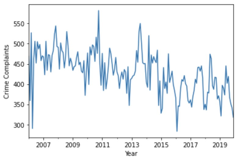
Visualizing your dataframes is also easy with MatPlotLib. Here we plot a simple line graph of the monthly aggregates from 2006 onwards:
monthly_df = monthly_df.set_index('timestamp')
ts = monthly_df['count']
ax = ts['2006':].plot()
ax.set_xlabel('Year')
ax.set_ylabel('Crime Complaints')
ax.set_xlabel('Year')
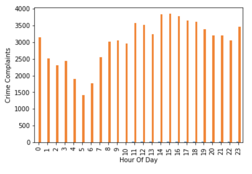
Likewise, it also simple to show the daily distribution by the hour in which crimes were reported:
ax = hourly_df.plot.bar()
ax.set_xlabel('Hour Of Day')
ax.set_ylabel('Crime Complaints')
ax.get_legend().remove()
plt.show()
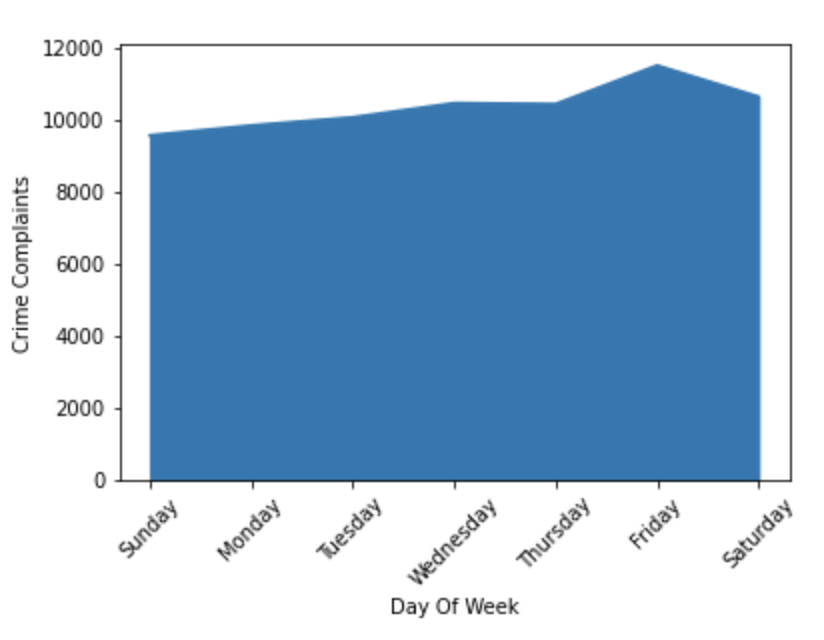
Showing the weekly distribution is a bit trickier as the Days of Week are not in comparitive order but creating a dictionary with the correct order and setting the index by that dictionary solves the problem.
order = ['Sunday', 'Monday', 'Tuesday', 'Wednesday','Thursday','Friday','Saturday']
ax = weekly_df.set_index('timestamp').loc[order].plot(kind='area')
ax.set_xlabel('Day Of Week')
ax.set_ylabel('Crime Complaints')
plt.xticks(rotation=45)
ax.get_legend().remove()
plt.show()
Conclusion
Pandas Dataframes are the perfect compliment to GridDB and can easily allow developers to quickly deploy data driven applications or, when combined with mathplotlib, gain new insights into their data without having to write tedious data transformations. What you trade for in raw read/write speed from a database perspective, you are more than likely to make up in ease of development and coding speed simply because dataframes provide a much more flexible and simpler way to analyze your large data sets.
The Jupyter Notebook used in this blog is available on the GridDB.net GitHub page here.