
Introduction
Today, we will be building a Bank Loan Classification model from scratch using the data stored in GridDB. In this post, we will cover the following:
1. Storing the data in GridDB
2. Extracting the data from GridDB
3. Building a Logistic Regression Model using Pandas
4. Evaluating our model using heat map and correlation matrix
We will begin with installing the prerequisites and setting up our environment. We will be using GridDB’s Python connector for this tutorial as the primary language used to model building is Python. GridDB has an extensive range of connecting libraries and APIs which makes it easier to deal with both SQL and NoSQL interface.
Environment and Prerequisites
The following tutorial is carried out on Ubuntu Operating system (v. 18.04) with gcc version 7.5.0., GridDB (v. 4.5.2) and Jupyter Notebooks (Anaconda Navigator). As the code is in Python 3, it can be executed on any device/code editor operating on the said programming language. In case, you are new to Python and Machine Learning, the following links would help you with the installation:
GridDB can be installed using their comprehensive guide available on Github. Prerequisites for GridDB’s python-connector include: 1. GridDB C-client 2. SWIG 3. pcre
Tutorial on Python-client installation can be found here
Dataset
For this tutorial, we will be working with a Bank Loan Classification dataset which is publicly available on Kaggle. There are a total of 5000 instances in the dataset along with 14 attributes. The attributes signify user data evaluated on various criteria such as income, age, experience, etc. The response variable, in this case, is the ‘Personal Loan’ variable which is binary in nature. A label of 0 implies a rejection of the loan application whereas 1 conveys an acceptance.
The objective is to classify an instance in either of those categories – 0 or 1 (rejected or accepted) based on the rest of the explanatory variables. This is a two-class classification task that could be accomplished using a Logistic Regression Model. So let’s dive right in!
Set the necessary paths
The following code needs to be executed in the Ubuntu Terminal or whichever Operating System you are using after you have installed GridDB and the pre-requisites mentioned above.
export CPATH=$CPATH:<Python header file directory path>

export PYTHONPATH=$PYTHONPATH:<installed directory path>

export LIBRARY_PATH=$LIBRARY_PATH:C client library file directory path
Importing necessary libraries
The first step is, of course, importing the necessary libraries. The libraries we will be using for this tutorial are as follows:
Note that you might encounter an installation error if you’re using these libraries for the first time. Try pip install package-name or conda install package-name.
Once the installation of these libraries is complete, we shall now import the griddb_python library. You could run the following command individually on the python console or create a .py file at your convenience. If the installation is successful, the import command should not return any error.
import griddb_python
Troubleshooting: It is possible that the build might not be successful. Run the make command after setting up the paths. You could also run a sample program to figure out the specifics.
Adding data to GridDB
import griddb_python as griddb
import pandas as pd

factory = griddb.StoreFactory.get_instance()

# Container Initialization
try:
    gridstore = factory.get_store(host=your_host, port=ypur_port,
            cluster_name=your_cluster_name, username=your_username,
            password=your_password)

    conInfo = griddb.ContainerInfo("Dataset_Name",
                    [["attribute1", griddb.Type.INTEGER],["attribute2",griddb.Type.FLOAT],
                    ....],
                    griddb.ContainerType.COLLECTION, True)

    cont = gridstore.put_container(conInfo)
    cont.create_index("id", griddb.IndexType.DEFAULT)

    dataset = pd.read_csv("BankLoanClassification.csv")

    #Adding data to container
    for i in range(len(dataset)):
        ret = cont.put(data.iloc[i, :])
    print("Data has been added")

except griddb.GSException as e:
    for i in range(e.get_error_stack_size()):
        print("[", i, "]")
        print(e.get_error_code(i))
        print(e.get_location(i))
        print(e.get_message(i))
Things to note 1. Replace the parameters of factory.get_store() function with your cluster credentials. Alternatively, see how to create a new cluster 2. Pass the relevant attribute name, dataset name and, data types to the function griddb.ContainerInfo()
Accessing data from GridDB using SQL
The griddb_python library allows the user to access the data via SQL in Python. This helps us use both languages to our advantage. We can now access what is stored in the database simply by passing a query within our python file like
statement = ('SELECT * FROM Dataset_Name')
sql_query = pd.read_sql_query(statement, cont)
Note that the pd.read_sql_query() function converts the data from the SQL query into a pandas dataframe. You can then directly work on the dataframe and build your machine learning model. Alternatively, you can import a csv file directly like:
import os
import numpy as np
import pandas as pd
import matplotlib.pyplot as plt
from sklearn.metrics import confusion_matrix,mean_squared_error,accuracy_score
from sklearn.preprocessing import MinMaxScaler
from sklearn.model_selection import train_test_split
from sklearn.preprocessing import StandardScaler
from sklearn.linear_model import LogisticRegression
from sklearn.metrics import accuracy_score
import seaborn as sns
import matplotlib.pyplot as plt
APP_PATH = os.getcwd()
APP_PATH
'C:\Users\SHRIPRIYA\Desktop\GridDB'
Loading our dataset
Note that if you have loaded your dataset using GridDB’s python_client, you can skip this step as it is redundant.
The APP_PATH variable contains the current directory which is appended to the file name in the below command. To avoid any complications, make sure that the python file and the csv file are in the same directory. If the case is otherwise, provide the full path of the dataset file to avoid FileNotFoundError
dataset = pd.read_csv(os.path.join(APP_PATH, 'UniversalBank.csv'))Exploring the dataset
We will be executing some trivial commands to get an overview of our dataset before building a model. Preprocessing and Analysis of your data is a good practice to ensure a more robust and effective model. The head command returns the first 5 rows of the dataset. In case, you want to display more, pass a number as an argument to the head command. For instance, dataset.head(20) would result in the first 20 rows whereas dataset.head(-5) would return the last 5.
dataset.head()
| ID | Age | Experience | Income | ZIP Code | Family | CCAvg | Education | Mortgage | Personal Loan | Securities Account | CD Account | Online | CreditCard | |
|---|---|---|---|---|---|---|---|---|---|---|---|---|---|---|
| 0 | 1 | 25 | 1 | 49 | 91107 | 4 | 1.6 | 1 | 0 | 0 | 1 | 0 | 0 | 0 |
| 1 | 2 | 45 | 19 | 34 | 90089 | 3 | 1.5 | 1 | 0 | 0 | 1 | 0 | 0 | 0 |
| 2 | 3 | 39 | 15 | 11 | 94720 | 1 | 1.0 | 1 | 0 | 0 | 0 | 0 | 0 | 0 |
| 3 | 4 | 35 | 9 | 100 | 94112 | 1 | 2.7 | 2 | 0 | 0 | 0 | 0 | 0 | 0 |
| 4 | 5 | 35 | 8 | 45 | 91330 | 4 | 1.0 | 2 | 0 | 0 | 0 | 0 | 0 | 1 |
Let’s check out the total length of the dataset which would later be split into testing and training.
len(dataset)5000
The dataset.dtypes command tells us what kind of datatype each attribute has. This step is essential as we will have to scale numeric variables and in cases of text data, we will need to create dummy variables or use an encoding scheme. Therefore, it is a good idea to get a look at our data so that we could plan these steps prior to model building
dataset.dtypesID int64
Age int64
Experience int64
Income int64
ZIP Code int64
Family int64
CCAvg float64
Education int64
Mortgage int64
Personal Loan int64
Securities Account int64
CD Account int64
Online int64
CreditCard int64
dtype: object
It is now time to check for missing values in the dataset. isnull() command returns True if there is at least one null value in the dataset. Null values are either deleted or replaced by a predecided value before passing the dataset for training. Fortunately, as there are no null values in our case, we will simply move forward. However, to get a total count of null values in your dataset, you can type dataset[key].isnull().sum(). [key] is the attribute name you are interested in. The dataset.dropna() command will drop any row containing atleast one null value.
dataset.isnull().values.any()False
We will be dropping the columns – ID and ZIP Code as they play little to no role in predicting a loan application outcome.
dataset.drop(["ID","ZIP Code"],axis=1,inplace=True)Displaying the columns to verify the previous step
dataset.keys()Index(['Age', 'Experience', 'Income', 'Family', 'CCAvg', 'Education',
'Mortgage', 'Personal Loan', 'Securities Account', 'CD Account',
'Online', 'CreditCard'],
dtype='object')
It is imperative to convert the ordinal data into dummy data before moving on to creating a model. This makes it easier for the model to interpret these attributes. We will leave out the numerical data as they are taken as-is by the model.
cat_cols = ["Family","Education","Personal Loan","Securities Account","CD Account","Online","CreditCard"]
dataset = pd.get_dummies(dataset,columns=cat_cols,drop_first=True,)dataset.keys()Index(['Age', 'Experience', 'Income', 'CCAvg', 'Mortgage', 'Family_2',
'Family_3', 'Family_4', 'Education_2', 'Education_3', 'Personal Loan_1',
'Securities Account_1', 'CD Account_1', 'Online_1', 'CreditCard_1'],
dtype='object')
We can see 3 dummy columns are created for the Family attribute. Similarly, for Education, Personal Loan, etc. The number of columns depends on the labels a particular attribute has. To put it simply, if a variable has 3 levels – 0,1,2, the number of dummy columns created will be 3.
Now our data is ready to be split into X and Y – Independent variables and the response variable. y will contain the labels, which in our case is the attribute – Personal_Loan_1.
X = dataset.copy().drop("Personal Loan_1",axis=1)
y = dataset["Personal Loan_1"]
Let’s see how many labels we have of each category
dataset["Personal Loan_1"].value_counts()0 4520
1 480
Name: Personal Loan_1, dtype: int64
sns.countplot(x ='Personal Loan_1', data=dataset, palette='hls')
plt.show()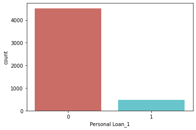
Splitting the dataset into Test and Train
Let us now split our dataset into Training and Testing. We have used an 80-20 ratio in our case. You could also use a 66-33 configuration which is more common. However, 1000 instances seem enough for training in this case.
trainx, testx, trainy, testy = train_test_split(X, y, test_size=0.20)print(trainx.shape)
print(testx.shape)
print(trainy.shape)
print(testy.shape)(4000, 14)
(1000, 14)
(4000,)
(1000,)
Scaling the features
Data Normalization or standardization is often performed when dealing with numeric data. This is important to ensure that each attribute lies within the same range. Data Standardization means rescaling the dataset such that it has an overall average of 0 and a standard deviation of 1. We will be using scikit-learn StandardScaler() for our purpose.
scaler = StandardScaler()
scaler.fit(trainx.iloc[:,:5])

trainx.iloc[:,:5] = scaler.transform(trainx.iloc[:,:5])
testx.iloc[:,:5] = scaler.transform(testx.iloc[:,:5])
C:UsersSHRIPRIYAanaconda3libsite-packagespandascoreindexing.py:966: SettingWithCopyWarning:
A value is trying to be set on a copy of a slice from a DataFrame.
Try using .loc[row_indexer,col_indexer] = value instead
See the caveats in the documentation: https://pandas.pydata.org/pandas-docs/stable/user_guide/indexing.html#returning-a-view-versus-a-copy
self.obj[item] = s
Building our Model
Now that our dataset is done with preprocessing, splitting and, standardizing, it is now time to pass it to the classification model. The training set and the output labels are passed to model.fit function for model building.
X = trainx
y = trainy

model = LogisticRegression()
model.fit(X , y)
predicted_classes = model.predict(X)
accuracy = accuracy_score(y,predicted_classes)
parameters = model.coef_
Model Evaluation
Accuracy and Coefficients
The accuracy here is training accuracy and parameters are the coefficients of the built model.
print(accuracy)
print(parameters)
print(model)
0.9615
[[-0.11052202 0.21417872 2.70013875 0.30873518 0.04262124 -0.19654911
1.68376406 1.39637464 3.44973088 3.7034019 -0.56957366 3.35123915
-0.64710272 -0.72719671]]
LogisticRegression()
Let us pass the test dataset to evaluate the accuracy of our model on unseen data of 1000 instances.
model.fit(testx , testy)
predicted_classes_test = model.predict(testx)
accuracy = accuracy_score(testy,predicted_classes_test)
print(accuracy)
0.962
Confusion Matrix and Heat Map
A confusion matrix shows 4 categories: 1. True Negative: Zeros predicted correctly (Actual and Predicted – 0) 2. False Negative: Ones wrongly predicted as zeros (Actual – 1, Predicted – 0) 3. False Positive: Zeros wrongly predicted as zeros (Actual – 0, Predicted – 1) 4. True Positive: Ones predicted correctly (Actual and Predicted – 1)
cm = confusion_matrix(testy,predicted_classes_test)
fig, ax = plt.subplots(figsize=(6, 6))
ax.imshow(cm)
ax.grid(False)
ax.xaxis.set(ticks=(0, 1), ticklabels=('Predicted 0s', 'Predicted 1s'))
ax.yaxis.set(ticks=(0, 1), ticklabels=('Actual 0s', 'Actual 1s'))
ax.set_ylim(1.5, -0.5)
for i in range(2):
    for j in range(2):
        ax.text(j, i, cm[i, j], ha='center', va='center', color='red')
plt.show()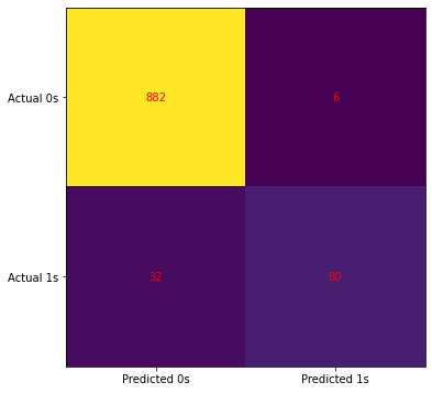
Conclusion and Future Scope
Our Bank Classification model achieved an accuracy of 95.3% on a dataset of 5000 instances which seems decent. The confusion matrix also revealed the specifics of false negatives and positives. The other alternatives for better accuracy can include – Naive Bayes, KNN Classifier, Decision Trees, SVM, etc. Explore more on the dataset home page here.
In this tutorial, we saw how can we insert our data into GridDB and access it using the python-client. We also used a simple SQL query to get the data from GridDB in a pandas dataframe. This ability of GridDB makes it versatile and thus, a popular choice for storing time-series data. There is a lot more you can do with GridDB. Check out our online community today!