Clustering Bustabit Gambling Behavior Using GridDB

Introduction

Understanding human behavior can be a tricky and attention-demanding task. It is not easy or simple to explain how people would act in a certain situation or how they make certain decisions. But observing people and trying to predict what they will do next can provide a real learning experience. It can help us to make an informed decision for better chances of a positive outcome.

One such situation where predicting human nature can be beneficial for observers is gambling. For instance, a game of poker – understanding why players raise, call, and fold in various situations can provide a distinct advantage competitively. In this project, we are going to use Bustabit data, an online platform for gamblers.

Rules for the game are as follows:

1. You can ‘Bet’ any amount in Bits, that is 1 millionth of a bitcoin
2. You can win if you cash out before the game busts
3. Your win calculated at the cash out according to the multiplier value at that moment
4. A percentage of ‘Bonus’ per game is applied to your bet and summed to give your final winning or ‘Profit’ in a winning game

We will be using GridDB to store our large amount of data, to access the data in real-time with fast processing.

Exporting and Import dataset using GridDB

GridDB is a highly scalable and optimized in-memory No SQL database that allows parallel processing for higher performance and efficiency, especially for time-series databases. We will be using GridDB’s python client, which allows us to connect GridDB to python and import or export data in real-time.

Libraries:

We will be using some python libraries to preprocess and analyze the data visually.

1. Pandas: Vastly used python library, especially when dealing with data frames.
2. Matplotlib: Primary library to present data visually using basic plots
3. Numpy: Library used to make some advanced mathematical calculations
4. Sklearn: Library that contains clustering algorithm that will be used in our project

Preprocessing:

data = pd.read_csv("bustabit.csv")

The dataset is now saved in the form of a data frame into the variable “data”.

To make our analysis more understandable, we will be adjusting a few columns of our dataset. We will be replacing the ‘ID’ column with a new one that acts as a primary key for our database. Also, we would be replacing ‘PlayDate’ with ‘Year’ because our project does not require any further information related to time.

data = data.drop(["Id"], axis = 1)
data.reset_index(drop=True, inplace=True)
data.index.name = 'ID'
    
data['Year'] = pd.DatetimeIndex(data['PlayDate']).year
data = data.drop('PlayDate', axis = 1)

These are the columns remaining in the data frame that we would be using in our analysis:

1. ID: Primary key for our database
2. GameID: Unique ID associated with the bustabit game
3. Username: Unique name used by the player on bustabit platform
4. Bet – The number of Bits betted by the player in this game
5. CashedOut – The multiplier at which this particular player cashed out
6. Bonus – The bonus reward (in percent) awarded to this player for the game
7. Profit – The amount this player won in the game, including the Bonus
8. BustedAt – The multiplier value at which this game busted
9. Year – The year in which the game was played

Before we export our database to GridDB, we need to deal with the NULL values present in our dataset, as GridDB does not allow null values in its database. We will be replacing the NULL values using the following rules:

1. CashedOut – If the value for ‘CashedOut’ is NA, we will set it to be 0.01 greater than the ‘BustedAt’ value to signify that the user failed to cash out before busting
2. Profit – If the value for Profit is NA, we will set it to be zero to indicate no profit for the player in that game
3. Bonus – If the value for Bonus is NA, we will set it to zero to indicate that there was no bonus for the player in that game.

data = data.assign(CashedOut = np.where((data['CashedOut'].isnull()),data['BustedAt'] + .01, data['CashedOut']))
data = data.assign(Profit = np.where((data['Profit'].isnull()), 0 , data['Profit']))
data = data.assign(Profit = np.where((data['Bonus'].isnull()), 0 , data['Bonus']))

As we have completed the preprocessing of our data, we can now save it on our local drive.

data.to_csv("preprocessed.csv")

Exporting Dataset into GridDB:

To upload the dataset to GridDB, we would read the CSV file that contains the preprocessed data.

data_processed = pd.read_csv("preprocessed.csv")

Now, we will create a GridDB container to pass our database schema to the GridDB to be able to generate the design of the database before inserting the row information. Next, we would insert our data into the GridDB.

#Create container 
data_container = "data_container"

# Create containerInfo
data_containerInfo = griddb.ContainerInfo(data_container,
                [["ID", griddb.Type.FLOAT],
                ["GameID", griddb.Type.FLOAT],
                ["Username", griddb.Type.STRING],
                ["Bet", griddb.Type.FLOAT],
                ["CashedOut", griddb.Type.FLOAT],
                ["Bonus", griddb.Type.FLOAT],
                ["Profit", griddb.Type.FLOAT],
                ["BustedAt", griddb.Type.FLOAT],
                ["Year", griddb.Type.INTEGER]],
                griddb.ContainerType.COLLECTION, True)
    
data_columns = gridstore.put_container(data_containerInfo)

print("container created and columns added")
    
# Put rows
data_columns.put_rows(data_processed)    
print("Data Inserted using the DataFrame")

We have now successfully exported the dataset to the GridDB platform.

Importing Dataset from GridDB:

To import the dataset from the GridDB platform, we will use TQL, GridDB’s query language similar to SQL. We will create a container and store the fetched data in it.

# Define the container names
data_container = "data_container"

# Get the containers
obtained_data = gridstore.get_container(data_container)
    
# Fetch all rows - language_tag_container
query = obtained_data.query("select *")

The next step would be to extract the rows in order of the column info and save it into a data frame to use for data visualization and analysis.

# Convert the list to a pandas data frame
data = pd.DataFrame(retrieved_data, columns=['ID', 'GameID',"Username",
                   "Bet","CashedOut" ,"Bonus", "Profit","BustedAt","Year"])

We now have our data saved into pandas data frame “data” and can continue to use it for our project.

Data Analysis

We will be using the Kmeans clustering algorithm to cluster the players into five different sets. We will start y introducing three new columns to understand the dataset even better. The new columns are based on the following rules:

1. Losses – If the new value for Profit is zero, we will set this to be the amount the player lost in that game, otherwise we will set it to zero. This value should always be zero or negative
2. GameWon – If the user made a profit in this game, the value should be 1, and 0 otherwise
3. GameLost If the user had a loss in this game, the value should be 1, and 0 otherwise

data = data.assign(Losses = np.where((data['Profit'] == 0 ), - data['Bet'], 0))
data = data.assign(GameWon = np.where((data['Profit'] == 0 ), 0 , 1))
data = data.assign(GameLost = np.where((data['Profit'] == 0 ), 1, 0))

Let’s take a look into some specific rows by filtering out data using conditions:

1. Highest multiplier: Details of the Game and User with highest ‘BustedAt’ value

data.iloc[data['BustedAt'].idxmax()]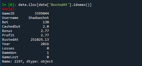

1. Highest Bet: Details of the Game and User with the highest Bet

data.iloc[data['Bet'].idxmax()]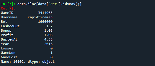

1. Highest Profit: Details of the Game and User with the highest Profit

data.iloc[data['Profit'].idxmax()]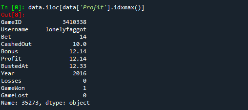

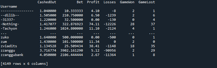
Next, we would group the data using ‘Username’ to identify the earnings, winnings, and losses by each user, throughout their gambling history at Bustabit. This would help us identify the gambling habits of each user and better understand of relationship and similarities between groups of players.

data_groupby = data.groupby('Username').agg({'CashedOut': 'mean',
                                             'Bet': 'mean',
                                             'Profit': 'sum',
                                             'Losses': 'sum',
                                             'GameWon': 'sum',
                                             'GameLost': 'sum'})

This is what our data looks like now:

Before moving unto clusters formation, we would first like to standardize the data across the dataset. This would transform the dataset into a standard measuring unit, making our algorithm more efficient. We will create our standardization function and apply it to every numerical column of our dataset.

def standardization_function(x):
    return (x-np.mean(x)/np.std(x))


bustabit_standardized = data_groupby.apply(lambda x: standardization_function(x) 
                                           if ((x.dtype == float) or (type(x) == int)) 

Our last step is to now form clusters of players into five sets using the sklearn library.

kmeans = KMeans(n_clusters=5, random_state=0).fit(bustabit_standardized)
clustering_data = pd.DataFrame()  
clustering_data['cluster'] = kmeans.predict(bustabit_standardized)

Here is a glimpse of our data divided into five clusters:

summary = clustering_data.groupby("cluster").mean()
summary['count'] = clustering_data['cluster'].value_counts()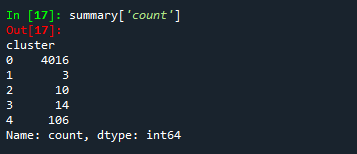

Conclusion

By looking at the final results of our project, we can conclude that most of the players have similar attributes and fall in the same clustering group while there are very few exceptions of players that are different from the standard behavior. All of the analysis was done using the GridDB database at the backend, making the integration seamless and efficient.

If you have any questions about the blog, please create a Stack Overflow post here https://stackoverflow.com/questions/ask?tags=griddb .
Make sure that you use the “griddb” tag so our engineers can quickly reply to your questions.