Create A Machine Learning Model using GridDB

Introduction

In this tutorial, we will build a trivial linear regression model with the data stored in GridDB. We will begin with GridDB’s python-connector to insert and access the data. Afterwards, we will see how to retrieve and convert the data using pandas and numpy. In the end, we will train and visualize our regression model using scikit-learn and matplotlib.

FULL SOURCE CODE

Prerequisites and Environment Setup

The following tutorial is carried out on Ubuntu Operating system (v. 18.04) with gcc version 7.5.0. GridDB (v. 4.5.2) has been installed using their documentation available on Github.

To enable the python connector for GridDB, prerequisites include GridDB C-client, SWIG and pcre. A detailed guide can be found here.

Set the necessary paths

export CPATH=$CPATH:<Python header file directory path>
export LIBRARY_PATH=$LIBRARY_PATH:<C client library file directory path>
export PYTHONPATH=$PYTHONPATH:<installed directory path>

Run the make command within the python-client directory. Install the necessary libraries.

$ pip3 install numpy
$ pip3 install pandas
$ pip3 install matplotlib

Run the following command within the python console to verify the installation

import griddb_python

Alternatively, you could execute one of the sample programs present in the /python-client/sample/ directory.

python3 sample1.py <GridDB notification address> <GridDB notification port> <GridDB cluster name> <GridDB user> <GridDB password>

→ Person: name=name02 status=False count=2 lob=[65, 66, 67, 68, 69, 70, 71, 72, 73, 74]

Note: You could run the aforementioned commands using just python and pip if your default Python version is already set to Python3. Ubuntu comes with a Python 2 default installation, therefore, we have explicitly mentioned python3 and pip3 while executing.

Accessing and retrieving data from GridDB

We would be using the publicly available CalCOFI dataset for this tutorial. It contains the time series data of oceanographic and larval fish in the world. The CalCOFI data has been inserted into the GridDB using the following command:

import griddb_python as griddb
import pandas as pd

factory = griddb.StoreFactory.get_instance()

# Initialize container
try:
    gridstore = factory.get_store(host=your_host, port=ypur_port, 
            cluster_name=your_cluster_name, username=your_username, 
            password=your_password)

    conInfo = griddb.ContainerInfo("Ocean_Data",
                    [["id", griddb.Type.INTEGER],["T_degC",griddb.Type.FLOAT],
                    ["Salnty", griddb.Type.FLOAT]],
                    griddb.ContainerType.COLLECTION, True)
    cont = gridstore.put_container(conInfo)   
    cont.create_index("id", griddb.IndexType.DEFAULT)
    data = pd.read_csv("bottle.csv")
    #Add data
    for i in range(len(data)):
        ret = cont.put(data.iloc[i, :])
    print("Data added successfully")

except griddb.GSException as e:
    for i in range(e.get_error_stack_size()):
        print("[", i, "]")
        print(e.get_error_code(i))
        print(e.get_location(i))
        print(e.get_message(i))

After the data insertion is successful, we can now access the data using SQL queries. 

sql_statement = ('SELECT * FROM Ocean_Data')
sql_query = pd.read_sql_query(sql_statement, cont)

The read_sql_query function offered by the pandas library converts the data fetched into a panda data frame to make it easy for the user to work.

sql_query.info()
<class 'pandas.core.frame.DataFrame'>

Linear Regression Model using CalCOFI Dataset

Due to the size of the CalCOFI dataset and for the sake of simplicity, we will be using the first 500 instances of this data to build a simple linear regression model.

The dataset contains 74 attributes or columns but for this tutorial, we would be using only 2 – Salinity and Temperature.
Let’s import all the necessary libraries

import numpy as np
import pandas as pd
from sklearn.model_selection import train_test_split
from sklearn.linear_model import LinearRegression
import matplotlib.pyplot as plt

We will now load our dataset. Make sure you keep the python file and the dataset within the same directory. Alternatively, supply the whole path of the csv file.
dataset = pd.read_csv(“bottle.csv”)

It is always a good idea to take a look at your dataset and get a gist of what you would be dealing with.

dataset.head()

Here’s the output:

To get the dimensions:

dataset.shape
Out []: (499, 74)

To get a deeper insight, let us describe our dataset

dataset.describe()

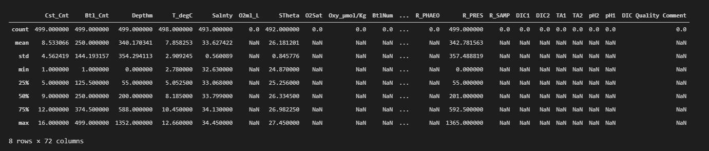
As mentioned above, we would only be using 2 attributes, so there is no need to keep the other attributes for this regression model.

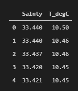
dataset=dataset[["Salnty","T_degC"]]
dataset.head()

Now our dataset displays only 2 attributes as expected.

Before training our model, it is always better to check for any missing or null values since they could hinder with the further procedure.

dataset.Salnty.isnull().value_counts()
Out[]: False    493
       True       6
       Name: Salnty, dtype: int64

dataset.T_degC.isnull().value_counts()
Out[]: False    498
       True       1
       Name: T_degC, dtype: int64

We will drop the null values and reset our index before moving to the training phase.

dataset=dataset.dropna(axis=0)
dataset.reset_index(drop=True,inplace=True)
dataset.shape
Out[]: (492,2)

Let us plot our dataset to see whether one varies with another.

plt.figure(figsize=(12,10))
plt.scatter(dataset.Salnty,dataset.T_degC, color='aqua')
plt.xlabel("Temperature",fontsize=22)
plt.ylabel("Salinity",fontsize=22)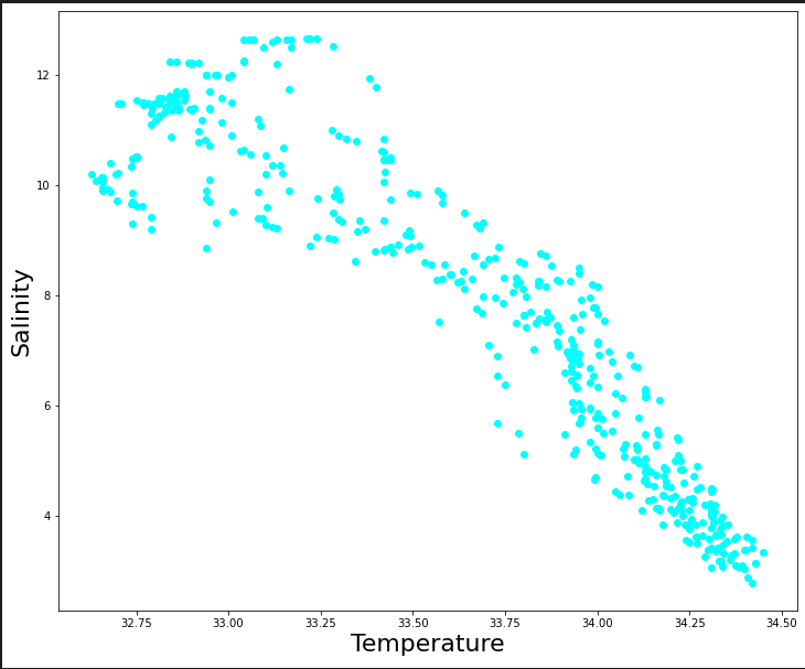

We will now reshape our data to a one-dimensional array.

x_label=np.array(dataset['Salnty']).reshape(492,1)
y_label=np.array(dataset['T_degC']).reshape(492,1)

It is now time to split our dataset to train and test. We will be using a 80%-20% scheme. Feel free to vary the proportions as per your convenience.

x_train, x_test, y_train, y_test = train_test_split(x_label, y_label, test_size = 0.2, random_state = 100)

Now that we have separated our dataset, it is time to build a linear regression model on our training dataset.

regression_model=LinearRegression()
regression_model.fit(x_train,y_train)
print('Coefficients: ', regression_model.coef_)
print('Intercept: ',regression_model.intercept_)

Out[]: Coefficients:  [[-4.80500593]]
       Intercept:  [169.4247854]

We will now supply our test dataset to check the accuracy of the built model.

accuracy = regression_model.score(x_test, y_test)
print(accuracy)
0.876504976866808

Let us visualize how well the line fits our data

plt.figure(figsize=(12,10))
plt.scatter(x_label, y_label,  color='aqua')
plt.plot(x_train, regression_model.predict(x_train),linewidth="4")
plt.xlabel("Temperature",fontsize=22)
plt.ylabel("Salinity",fontsize=22)
plt.title("Linear Regression",fontsize=22)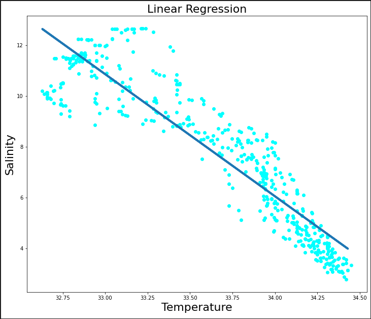

To check the mean error of our model

y_predicted_value = regression_model.predict(x_test)
print("Mean absolute error:",np.mean(np.absolute(y_predicted_value - y_test)))
Out []: Mean absolute error: 0.8090316355920698

In this tutorial, we saw how we can insert our data into GridDB and how it can be accessed using the pandas library and SQL. Later, we built a linear regression model out of this data. To connect GridDB with Jupyter notebooks, follow this tutorial.

Feel free to experiment with the other parameters of the dataset as well. For more such tutorials, check out our blog.

Source Code

Jupyter File

GitHub

If you have any questions about the blog, please create a Stack Overflow post here https://stackoverflow.com/questions/ask?tags=griddb .
Make sure that you use the “griddb” tag so our engineers can quickly reply to your questions.