Introduction and Purpose
New Series: A Python-Based IoT Data Dashboard
Many of the Internet of Things businesses are startups and have limited resources. But a cautious spending strategy never hurts even for a big corporation.
There are so many data visualization and real-time streaming tools around there. But, in fact, if all you need is a couple of charts that should be refreshed every two minutes, you do not have to spend your money on anything like that.
This article is the opening one of a series of three that we prepared for you. In this series, we will show you how to build a simple Python app that will pull the IoT data from GridDB and display three essential IoT metrics.
Based on the code we provide, you can create as many charts as you want, as well as customize them.
The series consists of the following tutorials: * scheduling the dashboard refresh * building a simple app with Python kivy * finalizing the app and adding the desktop icon
In the end, you will have a small but independent desktop application that you can start each morning and let it run during the day.
The app will show the data with the minimum time lag, almost in real-time actually, without any active participation on your side.
The Use Case
The article uses a test dataset that was created with the Python packages for generating random data. It imitates the standard connectivity data that would come from any IoT devices. Or, to be precise, the data that the SIM cards installed inside such devices send in the background.
Connectivity data is typically used by service engineers and support managers for troubleshooting and anomaly detection.
The Objectives
In this article, we will query the data and build three charts showing: * data usage * number of events * number of alerts
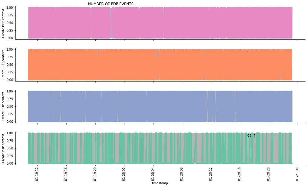
We will focus on the “Create PDP context†events as an example. Read more about PDP context here.
Then, we will make the query run every ten minutes and refresh the data accordingly.
Methods
To start, we will use Jupyter Notebook. You may as well run the final code in a Python IDE.
Prerequisites
One of the previous posts explains in detail how to query GridDB from a Jupyter Notebook.
Main Part
Preparations
Fetch the Data From the Database
To get the data from the database, we establish a connection with the jaydebeapi Python package and use an SQL-based query with a WHERE clause.
We used a GridDB-native function TIMESTAMP_ADD() to fetch only the data for the last hour. You can customize it as described in the GridDB SQL reference.
import pandas as pd
import jaydebeapi

conn = jaydebeapi.connect("com.toshiba.mwcloud.gs.sql.Driver",
                           "jdbc:gs://griddb:20001/defaultCluster/public?notificationMember:127.0.0.1:20001",
                           ["admin", "admin"],
                          "/usr/share/java/gridstore-jdbc-4.5.0.jar",)
iot = ('''SELECT

    TIMESTAMP(timestamp) as timestamp,
    event, simid, data_usage
FROM IoT

WHERE TIMESTAMP(timestamp) < TIMESTAMP_ADD(HOUR, NOW(), -1)''')
iotdf = pd.read_sql_query(iot, conn)
iotdf.head()| timestamp | event | simid | data_usage | |
|---|---|---|---|---|
| 0 | 2021-01-18 09:39:27.200000 | Create PDP context | 0003 | 0.00 |
| 1 | 2021-01-18 09:39:28.200000 | data | 0003 | 0.03 |
| 2 | 2021-01-18 09:39:29.200000 | Delete PDP context | 0003 | 0.00 |
| 3 | 2021-01-18 09:40:05.200000 | Create PDP context | 0003 | 0.00 |
| 4 | 2021-01-18 09:40:06.200000 | data | 0003 | 0.03 |
This is a time series dataset. It contains timestamps, events assigned to these timestamps, IDs of the SIM cards that sent the timestamps, as well as – where applicable – the amount of internet traffic, the data usage in kB.
Pivoting the data
In Jupyter, the timestamp column may sometimes appear as a string column in the data frame, even if it has a correct timestamp format in the database.
Convert it to the timestamp:
iotdf['timestamp']= iotdf['timestamp'].apply(pd.to_datetime)We have a so-called “slim” database that has few columns. We need to unfold or spread it first. We split the event column into a few more ones, one column per event type. If an event occurs, the respective column is filled with the value 1.
We transform the iot data frame into a pandas’ pivot table using the pivot_table() function.
pivotdf = iotdf.pivot_table(index=['timestamp', 'simid', 'data_usage'],
                                     columns='event',
                                     values= 'event',
aggfunc=lambda x: 1)pivotdf.head()| event | Create PDP context | Delete PDP context | alert | data | ||
|---|---|---|---|---|---|---|
| timestamp | simid | data_usage | ||||
| 2021-01-18 09:39:27.200 | 0003 | 0.00 | 1.0 | NaN | NaN | NaN |
| 2021-01-18 09:39:28.200 | 0003 | 0.03 | NaN | NaN | NaN | 1.0 |
| 2021-01-18 09:39:29.200 | 0003 | 0.00 | NaN | 1.0 | NaN | NaN |
| 2021-01-18 09:40:05.200 | 0003 | 0.00 | 1.0 | NaN | NaN | NaN |
| 2021-01-18 09:40:06.200 | 0003 | 0.03 | NaN | NaN | NaN | 1.0 |
Since the data frame has complex column names, and three columns are indexes now, we polish it to make it look like a normal data frame again. We drop the indexes with the reset_index() function.
Besides, we need to replace the NaNs with zero to be able to perform any calculations and actually plot the time series data. We use the fillna() function.
pivotdf = pivotdf.reset_index()
pivotdf = pivotdf.fillna(0)
pivotdf.head()
| event | timestamp | simid | data_usage | Create PDP context | Delete PDP context | alert | data |
|---|---|---|---|---|---|---|---|
| 0 | 2021-01-18 09:39:27.200 | 0003 | 0.00 | 1.0 | 0.0 | 0.0 | 0.0 |
| 1 | 2021-01-18 09:39:28.200 | 0003 | 0.03 | 0.0 | 0.0 | 0.0 | 1.0 |
| 2 | 2021-01-18 09:39:29.200 | 0003 | 0.00 | 0.0 | 1.0 | 0.0 | 0.0 |
| 3 | 2021-01-18 09:40:05.200 | 0003 | 0.00 | 1.0 | 0.0 | 0.0 | 0.0 |
| 4 | 2021-01-18 09:40:06.200 | 0003 | 0.03 | 0.0 | 0.0 | 0.0 | 1.0 |
Now, we are set to create visualizations.
Charts
We split each metric per device or SIM ID. It allows us to catch abnormalities in their behavior.
When it comes to creating grouped charts, the seaborn package has proven to be the fastest way. We do win a couple of seconds. It would not have been so important in any other situation. But if we want a real-time dashboard, we need our charts to be generated very quickly.
The seaborn package offers more than one opportunity to build grouped charts. We use the relational plot instead of the face grid, the second available option since the former works better with the line charts. And even though we have one event per timestamp, the line chart is a good choice to show continuity in the data. It also works better if we need to customize such chart parameters like the x-axis ticks rotations, etc.
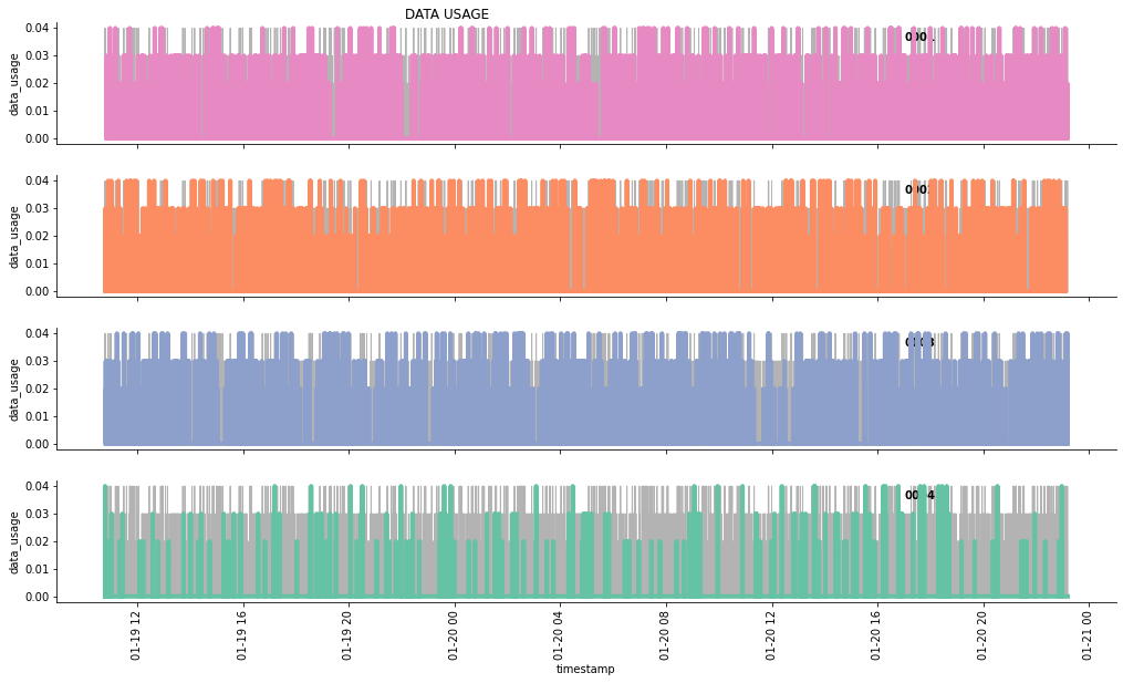
Below is an example with the data usage:
import seaborn as sns
import matplotlib.pyplot as plt

g = sns.relplot(
data=pivotdf, x="timestamp", y="data_usage", col="simid", hue="simid",col_order = ['0001', '0002', '0003', '0004'],
    kind="line", palette="Set2", linewidth=4, zorder=5,
    col_wrap=1, height=2, aspect=7, legend=False,
    )

for simid, ax in g.axes_dict.items():
    ax.text(.8, .85, simid, transform=ax.transAxes, fontweight="bold")

    sns.lineplot(data=pivotdf, x="timestamp", y="data_usage", units="simid",
            estimator=None, color=".7", linewidth=1, ax=ax,
        )

ax.set_xticks(ax.get_xticks()[::1])
g.set_xticklabels(rotation=90)

g.set_titles("")
g.fig.suptitle('DATA USAGE', horizontalalignment = 'right')
Text(0.5, 0.98, 'DATA USAGE')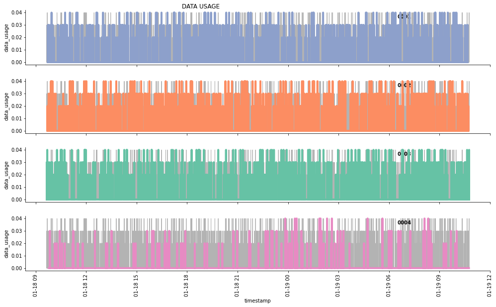
Creating the Automatic Refresh
Introducing the While Loop
We eventually arrive at the most exciting part!
All we need is to make the code run again and again without our active participation.
We use the while loop for this purpose. We simply wrap up the whole thing above in it (+ another two charts). And we start it once. Voalá! As long as your Jupyter Notebook or the Python IDE remains open and the script has been run once, it will continue to fetch the data and display refreshed charts.
A Few Optimization Remarks
Before sharing the complete code, a few best practices you need to know: * You definitely do not want to scroll through numerous identical charts. To spare yourself this effort, add the clear_output() into the loop, before anything else. * Since you cannot clear the output that does not exist, use try/except/pass to prevent the script from failing when it runs for the first time. * Optional: use try/except/pass for the charts that can have too little data to be rendered properly. It lets the script jump to the next section without breaking and throwing the error message. * Use the plt.show() function after each plot from the matplotlib package: otherwise, only the last plot in the code will be displayed. * Use the sleep() function at the end of each loop run to create a gap if it does not make sense to query the database in “real” real time. Give both your database and your CPU some breath. * Last but not least, add your custom status messages all over the code to watch the progress and do some troubleshooting. For instance, add print(“got new data”, datetime.now()) to mark when the new data was successfully fetched. Use datetime package to create your own timestamps.
There you go!
The Final Code
from datetime import datetime
from IPython.display import clear_output
import time
import seaborn as sns
import matplotlib.pyplot as plt
from PIL import Image, ImageDraw
import pandas as pd
import jaydebeapi
conn = jaydebeapi.connect("com.toshiba.mwcloud.gs.sql.Driver",
"jdbc:gs://griddb:20001/defaultCluster/public?notificationMember:127.0.0.1:20001",
["admin", "admin"],
"/usr/share/java/gridstore-jdbc-4.5.0.jar",)
curs = conn.cursor()
stop = 1
while stop > 0:
#delete the previous charts if any
try:
clear_output(wait=True)
except:
pass
#querying the data for the last hour
iot = ('''SELECT
TIMESTAMP(timestamp) as timestamp,
event, simid, data_usage
FROM IoT
WHERE TIMESTAMP(timestamp) > TIMESTAMP_ADD(HOUR, NOW(), -1)''')
iotdf = pd.read_sql_query(iot, conn)
print('got new data')
print(datetime.now())
#data preparation
iotdf['timestamp']= iotdf['timestamp'].apply(pd.to_datetime)
pivotdf = iotdf.pivot_table(index=['timestamp', 'simid', 'data_usage'],
columns='event',
values= 'event',
aggfunc=lambda x: 1)
pivotdf = pivotdf.reset_index()
pivotdf = pivotdf.fillna(0)
#data visualization
order = ['0001', '0002', '0003', '0004']
#data usage
g = sns.relplot(
data=pivotdf,
x="timestamp", y="data_usage", col="simid", hue="simid",col_order = ['0001', '0002', '0003', '0004'],
kind="line", palette="Set2", linewidth=4, zorder=5,
col_wrap=1, height=2, aspect=7, legend=False,
)
for simid, ax in g.axes_dict.items():
ax.text(.8, .85, simid, transform=ax.transAxes, fontweight="bold")
sns.lineplot(
data=pivotdf, x="timestamp", y="data_usage", units="simid",
estimator=None, color=".7", linewidth=1, ax=ax,
)
ax.set_xticks(ax.get_xticks()[::1])
g.set_xticklabels(rotation=90)
g.set_titles("")
g.fig.suptitle('DATA USAGE ', horizontalalignment = 'right')
plt.show()
#number of pdp events
g = sns.relplot(
data=pivotdf,
x="timestamp", y="Create PDP context", col="simid", hue="simid",col_order = ['0001', '0002', '0003', '0004'],
kind="line", palette="Set2", linewidth=4, zorder=5,
col_wrap=1, height=2, aspect=7, legend=False,
)
for simid, ax in g.axes_dict.items():
ax.text(.8, .85, simid, transform=ax.transAxes, fontweight="bold")
sns.lineplot(
data=pivotdf, x="timestamp", y="Create PDP context", units="simid",
estimator=None, color=".7", linewidth=1, ax=ax,
)
ax.set_xticks(ax.get_xticks()[::1])
g.set_xticklabels(rotation=90)
g.set_titles("")
g.fig.suptitle('NUMBER OF PDP EVENTS ', horizontalalignment = 'right')
plt.show()
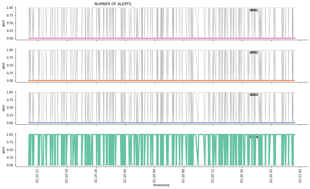
#alerts
g = sns.relplot(
data=pivotdf,
x="timestamp", y="alert", col="simid", hue="simid",col_order = ['0001', '0002', '0003', '0004'],
kind="line", palette="Set2", linewidth=4, zorder=5,
col_wrap=1, height=2, aspect=7, legend=False,
)
for simid, ax in g.axes_dict.items():
ax.text(.8, .85, simid, transform=ax.transAxes, fontweight="bold")
sns.lineplot(
data=pivotdf, x="timestamp", y="alert", units="simid",
estimator=None, color=".7", linewidth=1, ax=ax,
)
ax.set_xticks(ax.get_xticks()[::1])
g.set_xticklabels(rotation=90)
g.set_titles("")
g.fig.suptitle('NUMBER OF ALERTS ', horizontalalignment = 'right')
plt.show()
#putting it into sleep for 10 seconds
print('falling asleep')
print(datetime.now())
time.sleep(60)
got new data

2021-01-19 11:46:05.329856

falling asleep

2021-01-19 11:46:18.786249
Note
If you prefer to use Jupyter, you can expand the output section by clicking on it with the mouse and then using the CMD + O (the letter o).
Wait!
What about the while loop condition? Aren’t we going to descrease stop? Where does it come from, by the way?
No, we won’t descrease the stop variable. We do not want the loop to stop at all. You will stop it, when you close the Jupyter Notebook.
The condition was chosen arbitrarily. We just needed some random variable.
A Short Afterward
We have built an IoT connectivity data dashboard and make it refresh itself every ten seconds. Next time, we will integrate it into a small independent application.