Introduction
Each time you get an email alerting you about some unusual login activity in one of your online accounts, you’re seeing the process of anomaly detection in action.
Anomaly detection plays a key role in making sure modern systems run smoothly and securely, covering many different fields and use cases such as fraud detection, system health monitoring, intrusion detection, fault detection, quality assurance, and data mining.
In a nutshell, anomaly detection identifies unusual or unexpected patterns in datasets. These low-probability items or events are typically called outliers (although they’re also referred to as novelties in some contexts).
Machine learning techniques help automate the process of finding and handling outliers. This allows anomaly detection to run at scale and meet the demands of data-intensive, distributed systems like IoT and big data applications.
In this blog post, we’ll explore ways to use anomaly detection techniques in the popular Python library scikit-learn (sklearn) together with GridDB, an open-source IoT-optimized time-series database.
Some Preliminaries
Before we get started with anomaly detection in scikit-learn, let’s first go over some prerequisites we need to set up and a few things to keep in mind throughout our discussion.
Objectives and Scope
As mentioned earlier, this blog entry takes a look at the different anomaly detection tools and capabilities provided by the sklearn library, particularly when used together with gridDB. To get as good an overview and background as possible, we talk about both supervised and unsupervised anomaly detection with use cases ideal for working with both sklearn and GridDB.
Also, to keep our discussion straightforward and centered on this objective, we’ll focus our code examples on interfacing with GridDB, basic exploratory data analysis, and model training. We’ll be skipping on other steps in the machine learning pipeline such as feature selection, hyperparameter tuning, and model selection (although we’ll include key ideas and concepts for these topics as well).
Setting Up and Connecting to GridDB
We won’t go into detail on how to install and configure GridDB here. But if you want to follow along, check out this useful guide on setting up GridDB and connecting via Python . Also, we suggest using this docker-compose file to quickly get up and running with GridDB and Jupyter.
We also wrote a helper function to create a GridDB connection. The code is based on the previously-mentioned guides and is saved in a file utils/helpers/db.py in the project directory:
$ sudo yum -y install griddb_nosql griddb-c-clientimport jaydebeapi
def get_connection() -> jaydebeapi.Connection:
conn = jaydebeapi.connect(
"com.toshiba.mwcloud.gs.sql.Driver",
"jdbc:gs://griddb:20001/defaultCluster/public?notificationMember:127.0.0.1:20001",
["admin", "admin"],
"/usr/share/java/gridstore-jdbc-4.5.0.jar",
)
return connWith this function, we can obtain a GridDB connection in a Jupyter Notebook as well as in other scripts and modules used in this project (see next sections).
Data
We’re using two separate datasets for our scikit-learn anomaly detection overview. The first is an artificially-generated time series used in the unsupervised anomaly detection discussion, while the other contains labeled data used to train the supervised anomaly detection model.
Generating and Storing Artificial Sensor Data
For unsupervised anomaly detection, let’s create an artificial dataset that simulates output from an electricity usage sensor. The data points represent sensor readings (in Kilowatt-hours) taken at fixed time intervals. Here’s the function that does this:
import numpy as np
        import pandas as pd


        rng = np.random.RandomState(42)


        def create_sensor_data(
            size: int,
            freq: str,
            outlier_fraction: float
        ) -> pd.DataFrame:
            """Generates toy time-series dataset."""
            # Generate normally-distributed values
            ts_index = pd.date_range("2020-01-15", periods=size, freq=freq)
            sensor_readings = rng.normal(loc=4, scale=0.6, size=size)
            df = pd.DataFrame(sensor_readings, index=ts_index, columns=["kwh"])

            # Replace some values with outliers at random timestamps
            num_outliers = int(outlier_fraction * size)
            outlier_ts = np.random.choice(df.index, size=num_outliers, replace=False)
            df.loc[outlier_ts, "kwh"] = rng.normal(
                loc=9,
                scale=0.01,
                size=num_outliers
            )

            # Add integer timestamp column
            df['ts'] = df.apply(lambda row: int(row.name.timestamp()), axis=1)

            return df
The function returns a pandas DataFrame that contains a normally-distributed time series with outliers (values generated from a different distribution with mean several standard deviations away from the original).
For our discussion below, we generate 500 observations (2% of which are outliers) taken every 15 minutes:
sensor_data = create_sensor_data(
        size=500,
        freq='15T',
        outlier_fraction='0.02'
    )
We then store the time series into GridDB using the following function:
from jaydebeapi import Connection


        def load_into_sensor_table(conn: Connection, data: pd.DataFrame) -> int:
            """Inserts data into sensor table."""
            cursor = conn.cursor()
            row_count = 0

            try:
                # Create table
                cursor.execute(
                    """
                    CREATE TABLE IF NOT EXISTS power_sensor(
                        ts INTEGER PRIMARY KEY,
                        kwh FLOAT
                    )
                    """
                )

                # Insert all rows
                for row in data.itertuples():
                    cursor.execute(
                        """
                        INSERT INTO power_sensor(ts, kwh)
                        VALUES (?, ?)
                        """,
                        (row.ts, row.kwh)
                    )
                conn.commit()

                # Check if successfully inserted
                cursor.execute("SELECT * FROM power_sensor")
                result = cursor.fetchall()
                if len(result) == 0:
                    raise ValueError('No rows inserted')

                row_count = len(result)
            except Exception as e:
                conn.rollback()
                print(f'Error loading data into db: {e}')
            finally:
                cursor.close()

            return row_count
Here, we create a table called power_sensor and insert the values as rows. The value for the conn variable can be obtained using the get_connection() function we defined earlier as follows:
from utils.helpers.db import get_connection

        conn = get_connection()
        nrows = load_into_sensor_table(conn, sensor_data)
        nrows               # Should be 500 if everything is ok
Reading and Storing HTTP Request Data
For supervised anomaly detection, we use the http (KDDCUP99) dataset available from the Outlier Detection Datasets (ODDS) site. This dataset has the following details:
- contains 567,498 data points, each representing an HTTP request
- includes 3 attributes (duration, src_bytes, and dst_bytes)
- has label column that indicates whether a request is an attack (1) or normal traffic (0)
- applies log-transformation on the attributes to move original values away from zero
has 2,211 (0.4%) attacks (outliers)
It’s available as a downloadable .mat file, but isn’t readily readable using scipy.io.loadmat. So we need to use a package called mat7.3 to properly read the data into valid Python objects.
Once converted into a pandas DataFrame, we then store the data into GridDB via a similar function as the one used with the time series dataset. Here’s a snippet of that code:
# ...

        try:
            # Create table
            cursor.execute(
                """
                CREATE TABLE IF NOT EXISTS http_traffic(
                    duration FLOAT,
                    src_bytes FLOAT,
                    dst_bytes FLOAT,
                    is_attack INTEGER
                )
                """
            )

            # Insert all rows
            for row in data.itertuples():
                cursor.execute(
                    """
                    INSERT INTO http_traffic (duration, src_bytes, dst_bytes, is_attack)
                    VALUES (?, ?, ?, ?)
                    """,
                    (
                        row.duration,
                        row.src_bytes,
                        row.dst_bytes,
                        row.is_attack,
                    )
                )
            conn.commit()

    # ...
Detecting Anomalies with Sklearn
Sklearn ships with an extensive collection of machine learning models for doing both supervised and unsupervised anomaly detection. Let’s see some of the tools we can use and how we can apply them on data in GridDB.
Unsupervised Anomaly Detection
Unless we already have some prior knowledge of what “unusual†patterns in our data look like, we have to rely on unsupervised anomaly detection techniques to help us tell outliers apart from normal data points.
Unsupervised anomaly detection works by approximating a probability distribution which best represent the “normal†behavior of a dataset. Any data point that lies sufficiently far away from this distribution becomes a potential anomaly or outlier.
Different anomaly detection models use different ways to solve the above problem. In the scikit-learn library, these include density-based anomaly detection algorithms, cluster-based approaches, and support vector machine models.
Sklearn Models for Unsupervised Anomaly Detection
Some commonly-used unsupervised anomaly detection models in scikit-learn include:
- NearestNeighbors
- LocalOutlierFactor
- IsolationForest
- EllipticEnvelope
- KMeans
- DBSCAN
- TSNE
- OneClassSVM
Example Using IsolationForest
Now, let’s take a look at an example of unsupervised anomaly detection using sklearn’s IsolationForest model.
Isolation forest works by directly singling out specific outliers in the dataset instead of approximating how normal data points behave. It uses ensemble tree methods to isolate observations based on the idea that, since outliers are rare, they should take fewer splits to separate compared to normal observations. This places outliers closer to the root of the tree and thus require shorter average path lengths to traverse.
To see the isolation forest model in action, let’s use it to identify anomalies in our artificial sensor data.
Let’s begin with our imports:
import math

        import matplotlib.pyplot as plt
        import numpy as np
        import pandas as pd
        import seaborn as sns
        from sklearn.ensemble import IsolationForest
        from utils.helpers.db import get_connection
Recall that we stored the function get_connection() in a file located in ./utils/helpers/db.py (where ./ is the current directory containing this Jupyter notebook).
Below, we connect to our GridDB database and execute an SQL query that reads data from the power_sensor table:
conn = get_connection()
        sql_stmt = 'SELECT * FROM power_sensor'
        sensor_data = pd.read_sql(sql_stmt, conn)
Let’s get some info about the loaded dataset:
sensor_data.info()

        RangeIndex: 500 entries, 0 to 499
        Data columns (total 2 columns):
         #   Column  Non-Null Count  Dtype
        ---  ------  --------------  -----
         0   ts      500 non-null    int64
         1   kwh     500 non-null    float64
        dtypes: float64(1), int64(1)
        memory usage: 7.9 KB
Above, we see that the timestamp and electricity usage data have been correctly read into a DataFrame together with the correct column names and data types from the GridDB database.
To make our analysis and data visualization easier later, let’s set the timestamp as the index of the sensor_data DataFrame:
sensor_data.index = pd.to_datetime(sensor_data['ts'], unit='s')
We now explore the kwh (electricity usage) data a bit with some summary statistics, as well as get a feel for how it’s distributed with a run plot and box plot.
sensor_data.kwh.describe()
count 500.000000
mean 4.098142
std 0.908688
min 2.055240
25% 3.590052
50% 4.024251
75% 4.398410
max 9.019094
Name: kwh, dtype: float64
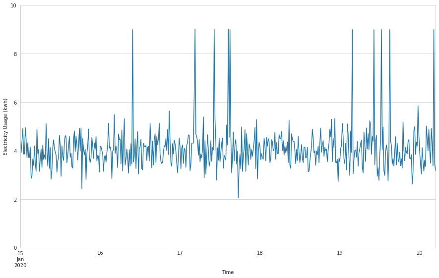
sensor_data.kwh.plot(
figsize=(15, 9),
ylim=(0, math.ceil(sensor_data.kwh.max())),
xlabel='Time',
ylabel='Electricity Usage (kwh)',
)
sensor_data.kwh.plot.box()
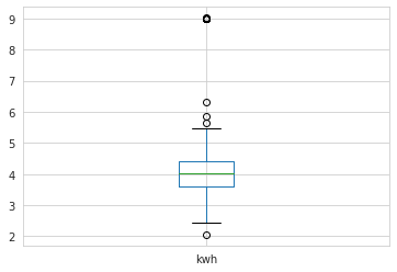
In the time series plot, we see sudden spikes in electricity usage at a few random points on the graph, indicating potential anomalies. When we examine this a bit closer with a box plot, we observe a number of points that lie beyond the whiskers, again indicating the presence of possible outliers.
Let’s now train an isolation forest model to see if it’s able to identify any outliers.
# Reshape the kwh time series into a 500 by 1 array
        kwh = sensor_data.kwh.values.reshape(-1, 1)

        # Fit the isolation forest model
        rng = np.random.RandomState(42)
        isolation_forest_clf = IsolationForest(
            contamination=0.02,
            max_samples=100,
            random_state=rng
        )
        isolation_forest_clf.fit(kwh)
        outlier_pred = isolation_forest_clf.predict(kwh)
In the preceding snippet, we first convert the kwh Series column into a numpy array with shape (500, 1) in order to be used later when fitting the model. We then create an instance of the IsolationForest model with the assumption that 2% of the kwh values are outliers. Next, we fit the model using values in the kwh array and finally apply the trained model to predict which kwh values are outliers and which ones aren’t.
The IsolationForest model’s predict() method returns an array of predicted values which are either -1 or 1. A value of -1 indicates that an observation is an outlier, while a value of 1 indicates a normal observation. It calculates an anomaly score for each observation, which is then used to determine whether the data point is an outlier or not.
Let’s set the outlier_pred array as a new column in sensor_data and see how many observations got labeled as outliers and how many were considered normal.
sensor_data['predicted_outlier'] = outlier_pred
sensor_data.predicted_outlier.value_counts()
1 490
-1 10
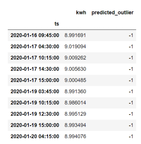
Name: predicted_outlier, dtype: int64Above, we see that the model classifies 10 data points as outliers and 490 as normal observations. Let’s see which ones are outliers:
sensor_data.loc[sensor_data.predicted_outlier == -1, ['kwh', 'predicted_outlier']]
To analyze the anomaly scores computed by our trained model, let’s follow a similar approach used in the official scikit-learn isolation forest example and borrow the code from this isolation forest tutorial. We can now visualize the anomaly score threshold and outlier region as follows:
plt.plot(xx, anomaly_score, label='Anomaly Score')
        plt.fill_between(
            xx.T[0],
            np.min(anomaly_score),
            np.max(anomaly_score),
            where=outlier==-1,
            color='r',
            alpha=.4,
            label='outlier region'
        )
        plt.legend()
        plt.ylabel('Anomaly Score')
        plt.xlabel('Electricity Usage (kwh)')
        plt.show();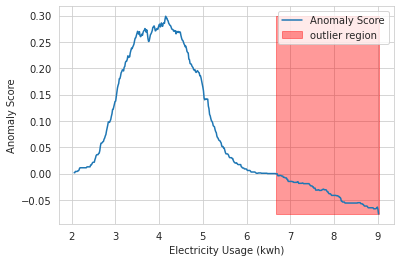
As we can observe, the trained isolation forest model correctly identifies all of the outliers we created from our artificial data generation procedure. But this comes with an important caveat that we know in advance what percentage of observations are actually outliers.
Supervised Anomaly Detection
When the dataset to analyze contains labels indicating which data points are outliers and which ones are normal observations, the anomaly detection process relies on classification techniques. Supervised classification models determine outliers by identifying relationships between features and labels.
In order for the model to correctly learn these relationships, it needs to be trained on a dataset with enough instances of outliers. However, since by nature outliers tend to be rare, this leads to the problem of imbalanced datasets. With imbalanced datasets, outliers get underrepresented during training, resulting in the model having poor recall of the anomaly class.
Sklearn Models for Supervised Anomaly Detection
Some popular scikit-learn models for supervised anomaly detection include:
- KNeighborsClassifier
- SVC (SVM classifier)
- DecisionTreeClassifier
- RandomForestClassifier
Example Using RandomForestClassifier
Let’s train an anomaly detection model that uses scikit-learn’s RandomForestClassifier to identify HTTP attacks. We use the http (KDDCUP99) dataset that we processed several sections ago.
For our supervised classification task, we import additional modules and functions from the scikit-learn library:
from sklearn.ensemble import RandomForestClassifier
        from sklearn.metrics import classification_report, confusion_matrix
        from sklearn.model_selection import train_test_split
Similar to our unsupervised anomaly detection example, we use the GridDB connection to fetch the data we need from the http_traffic table:
sql_stmt = 'SELECT * FROM http_traffic'

http_request_data = pd.read_sql(sql_stmt, conn)
Here’s what our dataset looks like overall:
        RangeIndex: 567498 entries, 0 to 567497
        Data columns (total 4 columns):
         #   Column     Non-Null Count   Dtype
        ---  ------     --------------   -----
         0   duration   567498 non-null  float64
         1   src_bytes  567498 non-null  float64
         2   dst_bytes  567498 non-null  float64
         3   is_attack  567498 non-null  int64
        dtypes: float64(3), int64(1)
        memory usage: 17.3 MB
We have the columns duration, src_bytes, and dst_bytes as our features, while the colum is_attack contains the labels (0 for normal HTTP request and 1 for HTTP attack).
Let’s see how many instances of HTTP attacks the dataset contains:
http_request_data.is_attack.value_counts()
        0    565287
        1      2211
        Name: is_attack, dtype: int64
There are a total of 2,211 outliers labeled here, or approximately 0.4% of all data points.
If we visualize the values for each of the attributes as box-and-whiskers plots categorized according to label, we see an interesting pattern:
http_request_data.boxplot(
        column=['duration', 'src_bytes', 'dst_bytes'],
        by='is_attack',
        figsize=(12, 8),
        layout=(3, 1)
    )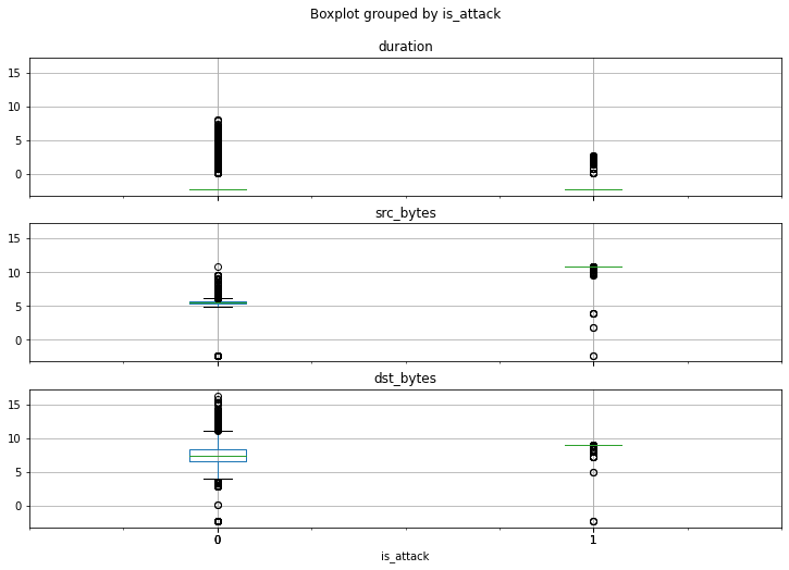
There’s a distinct difference in how the values for each of the three features are spread out when compared between outliers and non-outliers.
Next, let’s prepare our data for model fitting. We split our data into training and test sets below:
rng = np.random.RandomState(42)

        feature_cols = ['duration', 'src_bytes', 'dst_bytes']
        features = http_request_data[feature_cols]
        labels = http_request_data['is_attack']

        features_train, features_test, labels_train, labels_test = train_test_split(
            features,
            labels,
            stratify=labels,
            test_size=0.05,
            random_state=rng
        )
Above, we pass the values of the labels to the stratify parameter. This ensures that the proportions of the outlier and non-outlier classes are the same in both training and test datasets.
We’re now ready to fit the model and generate predictions:
random_forest_clf = RandomForestClassifier(n_jobs=4, random_state=rng)
        random_forest_clf.fit(features_train, labels_train)
        labels_pred = random_forest_clf.predict(features_test)
Let’s see how well the trained model performs by looking at the confusion matrix and the classification report:
print(confusion_matrix(labels_test, labels_pred))
        [[28264     0]
         [    0   111]]
    print(classification_report(labels_test, labels_pred))
                      precision    recall  f1-score   support

                   0       1.00      1.00      1.00     28264
                   1       1.00      1.00      1.00       111

            accuracy                           1.00     28375
           macro avg       1.00      1.00      1.00     28375
        weighted avg       1.00      1.00      1.00     28375
The results seem to show that the trained model does a very good job at identifying outliers and non-outliers. It got very high accuracy, precision, recall, and f1-score values. However, similar to our unsupervised anomaly detection example, we also need to be careful about accepting these numbers right away. This can indicate potential overfitting or another issue altogether. In real-world situations, this would just be part of a deeper analysis.
Conclusion
This blog post gave a short overview on the tools available in the scikit-learn library for doing anomaly detection. It also explained how to work with GridDB as a data source in sklearn-based machine learning projects using examples of supervised and unsupervised anomaly detection use cases. You’re now well equipped to explore sklearn’s anomaly detection capabilities further.