
Introduction
The Nobel Prize is perhaps the world’s most well-known and prestigious award. Professionals and activists from all over the world dream to become Nobel prize holders and share the prestige among the renowned advocates of their respective fields. Considering the significance and prestige of this award, business leaders and data analysts are excited to jump into the field and carry out exploratory and predictive analyses to find out the trend among the Nobel prize winners over the course of time.
Since these analyses that researchers and analysts are excited about are related to time-series activities, GridDB becomes the ideal choice for executing them as it is designed and optimized to deal with such time-series complexities.
The seamless integration of GridDB with Python offers a competitive advantage by leveraging the de facto leaders of the data science programming languages. In this article, we will use the power of GridDB – a highly scalable, in-memory NoSQL time-series database optimized for IoT and big data.
Without further ado, we will now take you through the step-by-step tutorial to get started with GridDB through a simple project aimed at visually analyzing the data available from The Nobel Foundation which includes the demographic data of all prize winners from the start of the prize, in 1901, to 2016. Let’s load it in and take a look.
Setting Up GridDB on Ubuntu
Before moving into the actual project and its implementation, make sure you have GridDB up and running on your system. For setting up GridDB on Ubuntu or CentOS, please refer to our detailed quick start guide for GridDB.
Dataset
For the purpose of this project, we will use the Nobel Laureates dataset publicly available on Kaggle.
Load File in DataFrame
To carry out exploratory and predictive analyses, Python offers an exceptional library, Pandas, that is specifically designed, implemented, and optimized to carry out data related complex tasks. Pandas have different modules that enable analysts and scientists to smoothly carry out the end-to-end process including the extraction of data from a CSV file.
# Read CSV file
nobelprize_data = pd.read_CSV("nobel.CSV")
In the above code snippet, we read from a CSV file and create Pandas data frames for further managing, transforming, and preprocessing the data.
Data Preprocessing
The data that we stored in Pandas data frame in the previous section will now be used for preprocessing. We will filter out data points relevant to our use-case, clean the data, and store the processed data into a new CSV file so that we do not end up running the preprocessing script again and again.
The CSV includes a number of columns that are not significant for our analysis and it would be better to have fewer columns to get a better insight into the data at this beginner stage.
# Drop irrelevant columns
nobelprize_data = nobelprize_data.drop(labels =
    ["Motivation","Full Name", "Birth Date",
    "Birth City" , "Birth Country",
    "Death Date", "Death City" , "Death Country" ,
    "Organization City", "Organization Country",
    "Organization Name"], axis = 1)
So, after removing few columns, we will have the following remaining columns:
- Year
- Category
- Prize (The title of the prize given to them)
- Prize Share (Date at which the prize was announced)
- Laureate ID (ID given by Nobel prize database)
- Laureate Type (If the Nobel prize was given to a group of people or individual person)
- Sex
Furthermore, it is also important to note that the columns are identified as non-null and in order to maintain the column, we need to make some changes in the ‘Sex’ column where the null represents ‘Not disclosed’
nobelprize_data['Sex'] = nobelprize_data['Sex'].fillna("Not disclosed")
Additionally, we will also introduce a column of ID to refer to it as the primary key for our database.
# Add auto incremental ID
nobelprize_data.index.name = 'ID'
Now we rename the column names to make them more comprehensive:
# Rename columns
fixColNames = nobelprize_data.rename(columns =
    {"Year": "year",
    "Category":"category",
    "Prize": "prize",
    "Prize Share":"prize_share",
    "Laureate ID":"laureate_id",
    "Laureate Type":"laureate_type",
    "Sex":"sex"})
After saving the processed data into the new CSV file, we will use the same procedure of loading the data from the CSV file into the Pandas data frame again.
# Generate a new processed file
fixColNames.to_CSV("preprocessed.CSV")
Once the data is loaded into the Pandas data frame, we are all set to insert it into GridDB to perform optimized analysis operations on the data.
Insert Data in GridDB
The standard approach set by GridDB to insert data is to create a container and use the put methods. We will combine this approach with Panda’s data insertion method in data frame.
First, we will instantiate a container, nobelprize_1901, in GridDB and define the data types. Please ensure that the data types are correct or you will likely run into validation errors while conducting analysis.
# Create Collection circuits
nobelprize_containerInfo = GridDB.ContainerInfo(nobelprize_container,
    [["ID", GridDB.Type.INTEGER],
    ["year", GridDB.Type.INTEGER],
    ["category", GridDB.Type.STRING],
    ["prize", GridDB.Type.STRING],
    ["prize_share", GridDB.Type.STRING],
    ["laureate_id", GridDB.Type.INTEGER],
    ["laureate_type", GridDB.Type.STRING],
    ["sex", GridDB.Type.STRING]],
    GridDB.ContainerType.COLLECTION, True)
nobelprize_columns = gridstore.put_container(nobelprize_containerInfo)
Now that a container is set up, we need to import our records into this container. The GridDB’s put_rows method allows us to import from data frames:
# Put rows
nobelprize_columns.put_rows(nobelprize_data)
The data and structure from the CSV are now successfully imported into the nobelprize_1901 and adapted to the GridDB structured format.
Access Data from GridDB
Now that the data is imported into the GridDB container, we need to retrieve it. GridDB has its own query language, TQL, which can be learnt about from this source. TQL is used to query data from the GridDB container and uses commands similar to the standard SQL protocol.
In this section, let’s see how to retrieve data from the Database. GridDB provides the query functionality which enables users to query the containers to retrieve data from the Database. Have a look at the following code block. There, we have retrieved the container using the get_container function and then querying the collection to extract the required data.
Here is a simple example of TQL we have used to retrieve the container using the get_container function and then extract the data using the query. In this particular case, we have used “ select * †to select all records from the container.
# Fetch all rows - circuits_container
query = nobelprize_data.query("select *")
For the scope and simplicity of this article, we have written a simple query to select all records. However, diving in further, you may explore using different commands to filter data along the lines of order, limits and conditions. Feel free to explore the syntax from the official GridDB sources mentioned earlier.
After fetching the data from the GridDB container, we need to import it back into the Pandas’ data frame for analysis. We achieve this using pd.DataFrame() method to convert the GridDB container lists to the data frame.
We now have a data frame fetched from the GridDB database.
Analysis in GridDB
Now that we have the dataset loaded into the GridDB container, it’s time to get onto the analysis. We will first import the required libraries: numpy, matplotlib, and pandas.
import numpy as np
import GridDB_python as GridDB
import sys
import pandas as pd
import matplotlib.pyplot as plt
We will now look into the Sex column of every Nobel Prize winner and generate a bar graph to contemplate the Sex: Nobel Prize ratio.
# Analysis on Gender
gender_wise = nobelprize_dataframe['sex'].value_counts()

genderplot = gender_wise.plot(kind='bar')
genderplot.figure.tight_layout()
genderplot.figure.savefig('gender_wise.png')
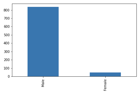
As is obvious, the Nobel Prize has been a male-dominated award. Reasons for this could be numerous, such as the lack of women empowerment in the early half of the 20th century. It could also be the case that there was a bias towards recognizing male talent as compared to females. In 2018, Donna Strickland was only the third woman to receive a Nobel prize in physics.
According to traditional stereotypes, women try to avoid STEM fields because they ‘don’t like maths’ or ‘are not good at science’. This is an ongoing issue to date, but for the past few decades, many efforts are made to overcome this view.
We notice that scientific fields have received the most recognition, amongst which Medicine and Physics stand out the most. It may be due to the fact that non-scientific fields in the 20th century were given less recognition or the Nobel Prizes for some fields either did not exist or were added later. A particular case is that of Computer Science which is not eligible for the Nobel Prize to date – they instead have another award called the Turing Award. If the aim of the analysis is to compare the recognition and popularity of disciplines, including the Turing Award would offer another meaningful insight (not covered in this article).
If we further analyse our data using both the previous categories into one graph.
# Analysis on Category
category_wise = nobelprize_dataframe['category'].value_counts()

nobelprize_dataframe.groupby(['category','sex']).size().unstack().plot(kind='bar',stacked=True)
plt.tight_layout()
plt.savefig('Category+Gender.png', orientation = 'landscape')
plt.show()
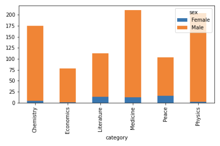
We can see that the only STEM field women recognition is somewhat notable is Medicine, while the overall most female Nobel prize winners contributed to the field of peace.
Another aspect that we can get some insight from is to analyse the awards given to each category over different time periods and how it has evolved over the years.
# Time series analysis on Year Group
nobelprize_dataframe["Year_Group"] = pd.cut(nobelprize_dataframe["year"],[1900,1910,1920,1930,1940,1950,1960,1970,1980,1990,2000,2010,2016], precision=0, labels=['1900-1910','1910-1920','1920-1930','1930-1940','1940-1950','1950-1960','1960-1970','1970-1980','1980-1990','1990-2000','2000-2010','2010-2016'])

nobelprize_dataframe.groupby(['Year_Group','category']).size().unstack().plot(kind='bar',stacked=True)
plt.tight_layout()
plt.savefig('Change_over_years.png')
plt.show()
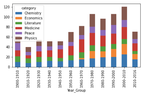
We can see in the graph below that there are some fields whose contribution remained constant over the past 120 years i.e Peace and Literature. While looking at the STEM areas of medicine and physics, we can clearly conclude that the Nobel prize contribution has increased significantly over the years. The most insight from the graphs is that the branch of Economics was invisible in the early 1900s but significant growth in the Nobel prizes awarded in Economics can be seen after 1970.
That’s it. We have learnt to load, insert, retrieve and analyze data using GridDB and Python.
Conclusion
In this article, we have created a simple project to get you started with GridDB. We have learnt how to pre-process and load a CSV file, insert and obtain data from GridDB containers and analyze data using matplotlib, pandas and numpy. We have also learnt the basics of querying data from GridDB and importing it into a dataframe.
This is just the beginning. Feel free to experiment more with TQL filters and GridDB containers to enrich your learning experience. Happy coding!