
Brain tumors are one of the most challenging diseases for clinical researchers, as it causes severe harm to patients. The brain is a central organ in the human body, and minor damage to this organ could affect the correct functioning of the human body. Brain tumors can lead to irreversible and dysfunctional damage to patients, including memory and vision loss. For these reasons, medical studies have, for a long time, focused on the study of the brain and its diseases, including brain tumors.
Computer studies have contributed to medical research by offering machine learning algorithms to classify medical analysis records as brain tumors or normal clinical conditions. This article presents the implementation of a brain tumor detection algorithm using machine learning techniques. For this purpose, the article begins by describing the environment, the dataset, and the necessary libraries. After that, the dataset is loaded and an exploratory data analysis is performed. The machine learning model is described and evaluated to obtain the results of the model.
The full Python jupyter file can be found here
Setting up your environment
To complete the use case presented in this article, it is necessary to prepare your environment. In this section, we present the environment and the context of execution of the proposed solution.
- Windows 10 is the operating system used in this article.
- Anaconda Navigator (Jupyter notebook). The Python code described in the article is executed in Jupyter notebook.
In later sections, we describe the use of GridDB to store the dataset used in this article. As we are using Python as our main programming language, we will need to prepare the environment to use GridDB with Python. For this purpose, we will need the following:
-
GridDB Python Client. The GridDB Python client allows communication with GridDB using Python.
GridDB Python Client is developed using:
— GridDB C Client
— SWIG (Simplified Wrapper and Interface Generator)
Introduction to the data
The dataset used in this article contains 7465 columns each corresponding to different measure units related to brain tumor detection, that are a result of medical analysis of patients. The dataset is composed of 35 entries each corresponding to a patient. The last column of the dataset is the y column and indicates, for each patient, the interpretation of the medical diagnosis of a brain tumor; normal or tumor. The dataset is available for the public and can be downloaded from Kaggle. Please download the dataset in order to fulfill the solution proposed in this article.
Importing the necessary libraries
First, we will need to handle the dataset. As detailed in later sections, this article provides two alternatives to load the dataset, using GridDB, or Panda to read the CSV file and provide an exploratory analysis of the dataset. For both cases, we will need to import the necessary libraries. Thanks to the Sklearn library the dataset is prepared to fit the machine learning model that is later evaluated thanks to the same library. The following cells in Jupyter Notebook import the necessary libraries used in this project:
import numpy as np
import pandas as pd
import matplotlib.pyplot as plt
from sklearn.metrics import confusion_matrix,accuracy_score
Loading the Dataset
In this section, two alternatives to load the dataset are provided; using GridDB, or using a CSV file. As described in earlier sections, the dataset used in this article is relatively extensive and might require a highly performant database for higher availability.
GridDB is a highly scalable, in-memory NoSQL time-series database optimized for IoT and Big Data. For these reasons, using GridDB to store our dataset can benefit our solution in different aspects. For the purpose of this article, we have already designed our database in GridDB and stored the dataset in a dedicated container. We will simply need to query the container in order to obtain our data. We perform this operation thanks to the following code:
import griddb_python as griddb

factory = griddb.StoreFactory.get_instance()

gridstore = factory.get_store(
    host="239.0.0.1",
    port=31999,
    cluster_name="defaultCluster",
    username="admin",
    password="admin"
)

col = gridstore.get_container("brain_tumor")

query = col.query("select *")
rs = query.fetch(False)
rows = rs.fetch_rows()
For more information on reading and writing data to GridDB using Python, an article is available on GridDB’s blog.
Alternatively, we can use the downloaded CSV file for the purpose of this article. Thanks to Pandas library we are able to read the data file.
dataset = pd.read_csv("data.csv")In the next section, we use the data obtained in the dataset variable to perform an exploratory data analysis.
Exploratory Data Analysis
The Pandas library offers a set of functions that will allow us to perform our exploratory data analysis. Some of these functions include the head(), columns, info(), and dtypes.
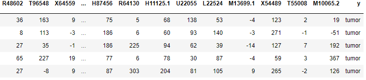
dataset.head()The previous line of code outputs an extract of the dataset providing 5 entries. This will allow us to have an overall look at our dataset.
We continue our exploratory data analysis to obtain the columns of the dataset:
dataset.columnsThis line of code outputs the following results:
Index(['Unnamed: 0', 'X53416', 'M83670', 'X90908', 'M97496', 'X90908.1', 'U37019', 'R48602', 'T96548', 'X64559', ... 'H87456', 'R64130', 'H11125.1', 'U22055', 'L22524', 'M13699.1', 'X54489', 'T55008', 'M10065.2', 'y'], dtype='object', length=7466)As we can observe, the last column of the dataset is the y columns, described in earlier sections. We can also notice that the number of columns is 7466, where one column corresponds to the ID column.
Now we will execute the info() function to our dataset:
dataset.info()This cell of code outputs the following results:
<class 'pandas.core.frame.DataFrame'>RangeIndex: 36 entries, 0 to 35Columns: 7466 entries, Unnamed: 0 to ydtypes: int64(7465), object(1)memory usage: 2.1+ MBThis output provides general information about the size, the data types, and the number of columns and rows present in the dataset.
In the Github repository for this article, we execute other functions to our dataset to complete our exploratory data analysis. Please check this repository for more details.
Machine Learning Model
This section describes the implementation of the machine learning model used in this article to classify the dataset entries. Before we get to this stage, we will need to make some operations in our dataset, including splitting the dataset.
We begin by assigning values to the X and y variables. In our case, the X variable will contain a slice of the dataset. The function iloc will return a dataframe; a 2-dimensional structured matrix representation of our dataset. In a similar way, the y variable will contain a series, which is a one-dimensional array. In our case, the y variable will contain the last column in the dataset. If we remember from earlier sections, the y column contains the actual interpretation of the brain tumor medical analysis; tumor or normal. This operation is achieved with the following lines of code:
X=dataset.iloc[:,:-1].values
y=dataset.iloc[:,-1].values
Now, we will need to encode the y categorical variable. This will transform the “Normal” and “tumor” values in the y column to 0s and 1s, respectively. We achieve this encoding thanks to the LabelEncoder.
from sklearn.preprocessing import LabelEncoder
le=LabelEncoder()
y=le.fit_transform(y)
At this point, we are ready to split our dataset into training data and test data. The training data will be used to train our model. The model will use this data in order to classify correctly the instances later on. We achieve this thanks to the following lines of code:
from sklearn.model_selection import train_test_split
X_train, X_test, y_train, y_test = train_test_split(X,y,test_size=.2,random_state=0)
Once we have performed these operations, we are ready to create our classification model. This is performed thanks to StandardScaler with the following lines of code:
from sklearn.preprocessing import StandardScaler
sc=StandardScaler()
X_train=sc.fit_transform(X_train)
X_test=sc.transform(X_test)
After that we choose the classification algorithm. In our case, we choose a logistic regression. Other algorithms are available including a k-nearest neighbor or a random forest classifier. Examples of these algorithms, and their corresponding results, are presented in the Github repository.
from sklearn.linear_model import LogisticRegression
classifier=LogisticRegression()
classifier.fit(X_train,y_train)
Model Evaluation
At this stage, we are ready to evaluate our model and obtain the results of the prediction using the test data. This is achieved thanks to the following lines of code:
y_pred_LogisticRegression=classifier.predict(X_test)
accuracy_score(y_test,y_pred_LogisticRegression)
The output of the prediction is 100%, meaning that the algorithm was able to correctly predict and classify all instances as having a brain tumor, or normal clinical conditions.
Conclusion
Machine learning studies can provide support systems for medical and clinical solutions. In this article, we provide a brain tumor detection model using machine learning, Python, and GridDB. For this purpose, we begin by setting up the environment to recreate the same context of execution. After that, we introduce the brain tumor dataset. The necessary Python libraries are imported. The dataset is loaded given two alternatives; using GridDB or a CSV file. An exploratory data analysis is performed. The dataset is also modified and made suitable for the machine learning model that is designed using logistic regression. The model is then evaluated and the results of the prediction are obtained.
The full Python jupyter file can be found here
References
https://www.kaggle.com/code/hisoka2020/brain-tumor-classification-accuracy-100/data