
The increasing use of smartphones has encouraged developers to create more and more mobile apps, on both platforms; android and ios. Around 70% of the mobile phones used by people are based on Android, making it more popular among people. In this project, we will be exploring data from the Google Play Store to gain insights regarding the apps and their popularity based on their specifications.
Exporting and Import dataset using GridDB
GridDB is a highly scalable and in-memory No SQL database that allows parallel processing for higher performance and efficiency, especially for our vast dataset. It is optimized for time-series databases for IoT and big data technologies. We can easily connect GridDB to python and use it to import or export data in real-time, with the help of the GridDB-python client.
Setup GridDB
First and foremost, we need to make sure that we have properly installed GridDB on our system. Our step-by-step guide available on the website can assist you with setting up GridDB on different operating systems.
Dataset
We will be using the dataset from the google play store stored in the CSV ‘apps.csv’. It contains all the details of the applications on Google Play. 13 features describe a given app, including its rating, size, and number of downloads.
Preprocessing
Before exporting the data to the GridDB platform, we will perform some preprocessing tasks to clean our data for optimal performance by GridDB. We will read the raw data available to us as CSV file.
apps_with_duplicates = pd.read_csv('datasets/apps.csv', index_col=0) We have our dataset saved as a dataframe to start the cleaning process. We would be removing some duplicates and null values from the apps dataset. We would also drop some columns that are not required for our analysis in this project and reset the index column to avoid discrepancies in our data.
apps = apps_with_duplicates.drop_duplicates()
apps.dropna(inplace=True)
apps.drop(['Genres','Content Rating', 'Last Updated', 'Current Ver', 'Android Ver'],axis = 1)
apps.reset_index(drop=True, inplace=True)
apps.index.name = 'ID'
The last step before storing the dataset is to remove the special characters from our dataset to be able to easily read our numerical data. We have a list of special characters already known that we would remove from our numerical columns.
# List of characters to remove
chars_to_remove = ['+', ',', 'M', '$']
# List of column names to clean
cols_to_clean = ['Installs', 'Size', 'Price']


# Loop for each column
for col in cols_to_clean:
    # Replace each character with an empty string
    for char in chars_to_remove:
        #print(col)
        #print(char)
        apps[col] = apps[col].astype(str).str.replace(char, '')
    apps[col] = pd.to_numeric(apps[col])
We will save the dataframes as local copies on our device before uploading them on GridDB.
apps.to_csv("apps_processed.csv")Exporting Dataset into GridDB:
Now we will upload the data to GridDB. For that, we will read the processed CSV files from the local drive and save them to different dataframes.
#read the cleaned data from csv
apps = pd.read_csv("apps_processed.csv")
Next, we will create a container to pass our column info of apps to the GridDB to be able to generate the design of the database before inserting the row information.
#Create container
apps_container = "apps_container"

# Create containerInfo
apps_containerInfo = griddb.ContainerInfo(apps_container,
                    [["ID", griddb.Type.INTEGER],
                    ["App", griddb.Type.STRING],
                    ["Category", griddb.Type.STRING],
                    ["Rating", griddb.Type.FLOAT],
                    ["Reviews", griddb.Type.FLOAT],
                    ["Size", griddb.Type.FLOAT],
                    ["Installs", griddb.Type.STRING],
                    ["Type", griddb.Type.STRING],
                    ["Price", griddb.Type.FLOAT]],
                    griddb.ContainerType.COLLECTION, True)

apps_columns = gridstore.put_container(apps_containerInfo)
After completing the schema, we will insert our row-wise data into the GridDB.
# Put rows
apps_columns.put_rows(apps)
The data is now successfully uploaded to the GridDB platform.
Importing Dataset from GridDB
We can easily extract the data from GridDB by creating the container and querying the relevant rows using TQL commands, a query language similar to SQL. We will use different containers and variables to store the two datasets separately.
# Define the container names
apps_container = "apps_container"

# Get the containers
obtained_apps = gridstore.get_container(apps_container)

# Fetch all rows - language_tag_container
query = obtained_apps.query("select *")

rs = query.fetch(False)
print(f"{apps_container} Data")

# Iterate and create a list
retrieved_data= []
while rs.has_next():
    data = rs.next()
    retrieved_data.append(data)

# Convert the list to a pandas data frame
apps = pd.DataFrame(retrieved_data, columns=["ID","App","Category","Rating","Reviews","Size","Installs","Type","Price"])

# Get the data frame details
print(apps)
apps.info()
Our data is now ready to be used for analysis.
Data Analysis and Visualization
We will start our analysis by exploring the dataset and understanding a few characteristics of the dataset.
- The Total number of distinct apps in our dataset
# Print the total number of apps
print('Total number of apps in the dataset = ', len(apps))![]()
- Most expensive app
Expensiveapp = apps.iloc[appdata['Price'].idxmax()]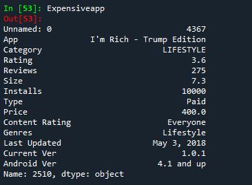
- Total number of categories in our dataset
# Print the total number of unique categories
num_categories = len(apps['Category'].unique())
print('Number of categories = ', num_categories)![]()
- Average app rating
avg_app_rating = apps['Rating'].mean()
print('Average app rating = ', avg_app_rating)![]()
We will continue our analysis by plotting some graphs against different specifications of an application. For example, we will start by dividing the apps into categories and then plotting the number of apps in each category to explore the most popular category among apps on the play store.
# Count the number of apps in each 'Category' and sort them in descending order
num_apps_in_category = apps['Category'].value_counts().sort_values(ascending = False)
num_apps_in_category.plot.bar()
plt.show()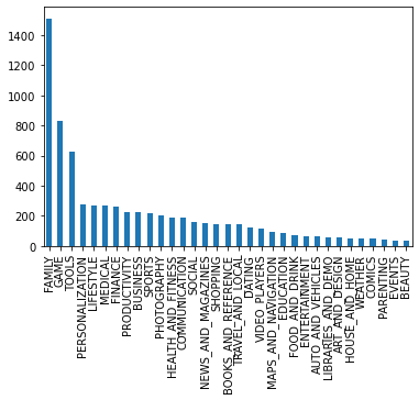
We can see that most of the applications belong to the ‘Family’ category. One of the reason for high number of applications in this category might be that it targets most of the audience and therefore they have higher chances of success in the market.
We would then use our dataset to gain insights about user preference for the cost of the app. There are two types of apps available on Google Playstore, mostly are free which means they cost $0, while some are paid apps. Let us compare the number of installs for paid applications vs free applications.
type_installs = apps[["Installs","Type"]].groupby(by = "Type").mean()
sns.barplot(data=type_installs, x=type_installs.index , y = "Installs" )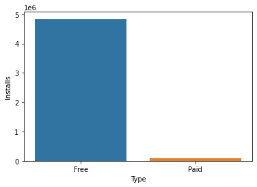
The results are as expected. People tend to download applications that are free and are usually reluctant to pay for them unless necessary.
We will compare the price of the app across different categories. Selecting a few popular categories out of our dataset then plotting it across the apps with prices lesser than $100 would give us a better understanding of the pricing strategy used while developing mobile applications, because most of the applications in our dataset lie below $100 and others would be considered as outliers.
# Select a few popular app categories
popular_app_cats = apps[apps.Category.isin(['GAME', 'FAMILY', 'PHOTOGRAPHY',
                                            'MEDICAL', 'TOOLS', 'FINANCE',
                                            'LIFESTYLE','BUSINESS'])]

# Select apps priced below $100
apps_under_100 = popular_app_cats[popular_app_cats['Price']<100]

fig, ax = plt.subplots()
fig.set_size_inches(15, 8)

# Examine price vs category with the authentic apps (apps_under_100)
ax = sns.stripplot(x='Price', y='Category', data=apps_under_100,
                   jitter=True, linewidth=1)
ax.set_title('App pricing trend across categories after filtering for outliers')
plt.show()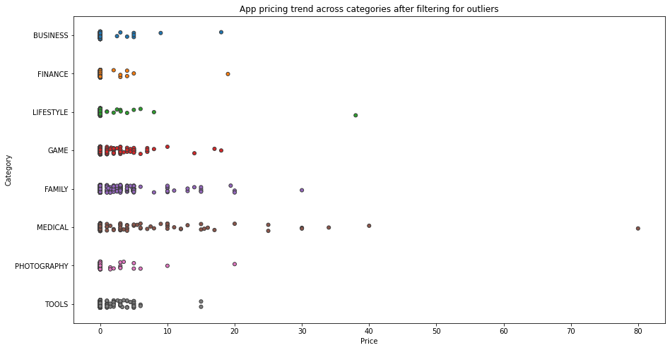
We can see that most of the expensive apps belong to the business or medical field, while apps belonging to games, tools, or photography categories lie under $20. This is because of the selected users for which the application is specified. Most of the games of tools or photography applications are designed for leisure purposes and people tend to think twice to spend money on these applications. They generate revenues mostly through ads and/or third-party collaborations.
Conclusion:
We can conclude that the developing application is as important as other aspects of the product management including setting the price and targeting the audience. All of the analysis was done using the GridDB database at the backend, making the integration seamless and efficient.
If you have any questions about the blog, please create a Stack Overflow post here https://stackoverflow.com/questions/ask?tags=griddb .
Make sure that you use the “griddb” tag so our engineers can quickly reply to your questions.