Multi Class Text Classification using Python and GridDB

On the Internet, there are a lot of sources that provide enormous amounts of daily news. Further, the demand for information by users has been growing continuously, so it is important to classify the news in a way that lets users access the information they are interested in quickly and efficiently. Using this model, users would be able to identify news topics that go untracked, and/or make recommendations based on their prior interests. Thus, we aim to build models that take news headlines and short descriptions as inputs and produce news categories as outputs.

The problem we will tackle is the classification of BBC News articles and their categories. Using the text as an input, we will predict what the category would be. There are five types of categories: business, entertainment, politics, sport, and technology.

The outline of the tutorial is as follows:

1. Prerequisites and Environment setup
2. Dataset overview
3. Importing required libraries
4. Loading the dataset
5. Data Cleaning and Preprocessing
6. Building and Training a Machine Learning Model
7. Conclusion

1. Prerequisites and Environment setup

This tutorial is carried out in Anaconda Navigator (Python version – 3.8.3) on Windows Operating System. The following packages need to be installed before you continue with the tutorial –

1. Pandas

2. NumPy

3. tensorflow

4. nltk

5. csv

6. griddb_python

7. matplotlib

You can install these packages in Conda’s virtual environment using conda install package-name. In case you are using Python directly via terminal/command prompt, pip install package-name will do the work.

GridDB installation

While loading the dataset, this tutorial will cover two methods – Using GridDB as well as Using Pandas. To access GridDB using Python, the following packages also need to be installed beforehand:

1. GridDB C-client
2. SWIG (Simplified Wrapper and Interface Generator)
3. GridDB Python Client

2. Dataset Overview

Text documents are one of the richest sources of data for businesses.

We’ll use a public dataset from the BBC comprised of 2225 articles, each labeled under one of 5 categories: business, entertainment, politics, sport or tech.

The dataset used in this project is the BBC News Raw Dataset. It can be downloaded from here (http://mlg.ucd.ie/datasets/bbc.html).

3. Importing Required Libraries

import griddb_python as griddb
import csv
import tensorflow as tf
import numpy as np
import pandas as pd
from tensorflow.keras.preprocessing.sequence import pad_sequences
from tensorflow.keras.preprocessing.text import Tokenizer
from tensorflow.keras.models import Sequential
from tensorflow.keras.layers import Dense, Flatten, LSTM, Dropout, Activation, Embedding, Bidirectional
import nltk
from nltk.corpus import stopwords
import matplotlib.pyplot as plt

4. Loading the Dataset

Let’s proceed and load the dataset into our notebook.

4.a Using GridDB

Toshiba GridDB™ is a highly scalable NoSQL database best suited for IoT and Big Data. The foundation of GridDB’s principles is based upon offering a versatile data store that is optimized for IoT, provides high scalability, tuned for high performance, and ensures high reliability.

To store large amounts of data, a CSV file can be cumbersome. GridDB serves as a perfect alternative as it in open-source and a highly scalable database. GridDB is a scalable, in-memory, No SQL database which makes it easier for you to store large amounts of data. If you are new to GridDB, a tutorial on reading and writing to GridDB can be useful.

Assuming that you have already set up your database, we will now write the SQL query in python to load our dataset.

sql_statement = ('SELECT * FROM bbc-text')
dataset = pd.read_sql_query(sql_statement, cont)

Note that the cont variable has the container information where our data is stored. Replace the bbc-text with the name of your container. More info can be found in this tutorial reading and writing to GridDB.

When it comes to IoT and Big Data use cases, GridDB clearly stands out among other databases in the Relational and NoSQL space. Overall, GridDB offers multiple reliability features for mission-critical applications that require high availability and data retention.

4.b Using With statement

In Python you need to give access to a file by opening it. You can do it by using the open() function. Open returns a file object, which has methods and attributes for getting information about and manipulating the opened file. Both of the above methods will lead to the same output as the data is loaded in the form of a pandas dataframe using either of the methods.

We import ntlk library and import the stopwords function. We will set the stopwords for English language. These are the samples for English stopwords: has, hasn’t, and, aren’t, because, each, during.

The process of converting data to something a computer can understand is referred to as pre-processing. One of the major forms of pre-processing is to filter out useless data. In natural language processing, useless words (data), are referred to as stop words.

A stop word is a commonly used word (such as “the”, “a”, “an”, “in”) that a search engine has been programmed to ignore, both when indexing entries for searching and when retrieving them as the result of a search query. We would not want these words to take up space in our database, or taking up valuable processing time. For this, we can remove them easily, by storing a list of words that you consider to stop words.

nltk.download('stopwords')
STOPWORDS = set(stopwords.words('english'))

#We populate the list of articles and labels from the data and also remove the stopwords.
articles = []
labels = []

with open("bbc-text.csv", 'r') as csvfile:
    reader = csv.reader(csvfile, delimiter=',')
    next(reader)
    for row in reader:
        labels.append(row[0])
        article = row[1]
        for word in STOPWORDS:
            token = ' ' + word + ' '
            article = article.replace(token, ' ')
            article = article.replace(' ', ' ')
        articles.append(article)

We set the hyper-Parameters that are required to build and train the model.

vocab_size = 5000 
embedding_dim = 64
max_length = 200
trunc_type = 'post'
padding_type = 'post'
oov_tok = '<oov>' # OOV = Out of Vocabulary
training_portion = 0.8</oov>

Once the dataset is loaded, let us now explore the dataset. We’ll print the first 10 rows of this dataset using head() function.

5. Data Cleaning and Preprocessing

articles[:1]

['tv future hands viewers home theatre systems  plasma high-definition tvs  digital video recorders moving living room  way people watch tv radically different five years  time.  according expert panel gathered annual consumer electronics show las vegas discuss new technologies impact one favourite pastimes. us leading trend  programmes content delivered viewers via home networks  cable  satellite  telecoms companies  broadband service providers front rooms portable devices.  one talked-about technologies ces digital personal video recorders (dvr pvr). set-top boxes  like us tivo uk sky+ system  allow people record  store  play  pause forward wind tv programmes want.  essentially  technology allows much personalised tv. also built-in high-definition tv sets  big business japan us  slower take europe lack high-definition programming. people forward wind adverts  also forget abiding network channel schedules  putting together a-la-carte entertainment. us networks cable satellite companies worried means terms advertising revenues well  brand identity  viewer loyalty channels. although us leads technology moment  also concern raised europe  particularly growing uptake services like sky+.  happens today  see nine months years  time uk   adam hume  bbc broadcast futurologist told bbc news website. likes bbc  issues lost advertising revenue yet. pressing issue moment commercial uk broadcasters  brand loyalty important everyone.  talking content brands rather network brands   said tim hanlon  brand communications firm starcom mediavest.  reality broadband connections  anybody producer content.  added:  challenge hard promote programme much choice.   means  said stacey jolna  senior vice president tv guide tv group  way people find content want watch simplified tv viewers. means networks  us terms  channels could take leaf google book search engine future  instead scheduler help people find want watch. kind channel model might work younger ipod generation used taking control gadgets play them. might suit everyone  panel recognised. older generations comfortable familiar schedules channel brands know getting. perhaps want much choice put hands  mr hanlon suggested.  end  kids diapers pushing buttons already - everything possible available   said mr hanlon.  ultimately  consumer tell market want.   50 000 new gadgets technologies showcased ces  many enhancing tv-watching experience. high-definition tv sets everywhere many new models lcd (liquid crystal display) tvs launched dvr capability built  instead external boxes. one example launched show humax 26-inch lcd tv 80-hour tivo dvr dvd recorder. one us biggest satellite tv companies  directtv  even launched branded dvr show 100-hours recording capability  instant replay  search function. set pause rewind tv 90 hours. microsoft chief bill gates announced pre-show keynote speech partnership tivo  called tivotogo  means people play recorded programmes windows pcs mobile devices. reflect increasing trend freeing multimedia people watch want  want.']

labels[:1]

    ['tech']

Now, let’s proceed to building and evaluating machine learning models on our credit card dataset. We’ll first create features and labels for our model and split them into train and test samples. Test size has been kept as 20% of the total dataset size.

We need to split them into training set and validation set. We set 80% (training_portion = .8) for training and another 20% for validation.

train_size = int(len(articles) * training_portion)

train_articles = articles[0: train_size]
train_labels = labels[0: train_size]

validation_articles = articles[train_size:]
validation_labels = labels[train_size:]

5.a Tokenization

Tokenization is set with num_words equal to vocab_size (5000) and oov_token equal to ‘‘. The method fits_on_texts is called on train_articles. By using word frequency, this method creates the vocabulary index. In the example given, “The cat sat on the mat. “, it will create a dictionary {‘‘: 1, ‘cat’: 3, ‘mat’: 6, ‘on’: 5, ‘sat’: 4, ‘the’: 2}.

tokenizer = Tokenizer(num_words = vocab_size, oov_token=oov_tok)
tokenizer.fit_on_texts(train_articles)
word_index = tokenizer.word_index

The oov_token is the value ‘’ that we put if the word is not listed in the dictionary.

5.b Convert to Sequences

Tokenization is followed by the method text_to_sequences. It converts each text in texts into an integer sequence. The method basically takes each word in the text and replaces it with its corresponding integer from the dictionary tokenizer.word_index. If the word is not in the dictionary, it will be assigned value of 1.

train_sequences = tokenizer.texts_to_sequences(train_articles)

5.c Sequence Truncation and Padding

When we train them for NLP, we need to make those sequences the same size (concrete shape). To make sure that all sequences are the same size, we will use padding and truncate them.

train_padded = pad_sequences(train_sequences, maxlen=max_length, padding=padding_type, truncating=trunc_type)

We will apply tokenization, convert to sequences and padding/truncating to train_articles and validation_articles.

tokenizer = Tokenizer(num_words = vocab_size, oov_token=oov_tok)
tokenizer.fit_on_texts(train_articles)
word_index = tokenizer.word_index

train_sequences = tokenizer.texts_to_sequences(train_articles)
train_padded = pad_sequences(train_sequences, maxlen=max_length, padding=padding_type, truncating=trunc_type)

validation_sequences = tokenizer.texts_to_sequences(validation_articles)
validation_padded = pad_sequences(validation_sequences, maxlen=max_length, padding=padding_type, truncating=trunc_type)

As before, we need to do the same thing here as we did with the features and articles. The model does not understand words, so we need to convert the label to numbers. We tokenize and convert to sequence the same as before. When doing the tokenization, we don’t indicate the vocab size and oov_token.

label_tokenizer = Tokenizer()
label_tokenizer.fit_on_texts(labels)

training_label_seq = np.array(label_tokenizer.texts_to_sequences(train_labels))
validation_label_seq = np.array(label_tokenizer.texts_to_sequences(validation_labels))

6. Machine Learning Model Building

Now we are ready to create the Neural Network model. The model architecture consist of the following layers:

model = Sequential()

model.add(Embedding(vocab_size, embedding_dim))
model.add(Dropout(0.5))
model.add(Bidirectional(LSTM(embedding_dim)))
model.add(Dense(6, activation='softmax'))

model.summary()

    Model: "sequential"
    _________________________________________________________________
    Layer (type)                 Output Shape              Param #   
    =================================================================
    embedding (Embedding)        (None, None, 64)          320000    
    _________________________________________________________________
    dropout (Dropout)            (None, None, 64)          0         
    _________________________________________________________________
    bidirectional (Bidirectional (None, 128)               66048     
    _________________________________________________________________
    dense (Dense)                (None, 6)                 774       
    =================================================================
    Total params: 386,822
    Trainable params: 386,822
    Non-trainable params: 0
    _________________________________________________________________

We then compile the model to configure the training process with the loss sparse_categorical_crossentropy since we didn’t one-hot encode the labels. We use Adam optimizer.

opt = tf.keras.optimizers.Adam(learning_rate=0.001, decay=1e-6)
model.compile(loss='sparse_categorical_crossentropy', optimizer=opt, metrics=['accuracy'])

num_epochs = 12
history = model.fit(train_padded, training_label_seq, epochs=num_epochs, validation_data=(validation_padded, validation_label_seq), verbose=2)

    Epoch 1/12
    56/56 - 8s - loss: 1.6055 - accuracy: 0.2949 - val_loss: 1.4597 - val_accuracy: 0.3191
    Epoch 2/12
    56/56 - 5s - loss: 1.0623 - accuracy: 0.5854 - val_loss: 0.7767 - val_accuracy: 0.8000
    Epoch 3/12
    56/56 - 5s - loss: 0.6153 - accuracy: 0.7989 - val_loss: 0.7209 - val_accuracy: 0.7910
    Epoch 4/12
    56/56 - 5s - loss: 0.3402 - accuracy: 0.9101 - val_loss: 0.5048 - val_accuracy: 0.8135
    Epoch 5/12
    56/56 - 6s - loss: 0.1731 - accuracy: 0.9685 - val_loss: 0.1699 - val_accuracy: 0.9618
    Epoch 6/12
    56/56 - 6s - loss: 0.0448 - accuracy: 0.9955 - val_loss: 0.1592 - val_accuracy: 0.9663
    Epoch 7/12
    56/56 - 6s - loss: 0.0333 - accuracy: 0.9966 - val_loss: 0.1428 - val_accuracy: 0.9663
    Epoch 8/12
    56/56 - 5s - loss: 0.0400 - accuracy: 0.9927 - val_loss: 0.1245 - val_accuracy: 0.9685
    Epoch 9/12
    56/56 - 6s - loss: 0.0178 - accuracy: 0.9972 - val_loss: 0.1179 - val_accuracy: 0.9685
    Epoch 10/12
    56/56 - 5s - loss: 0.0135 - accuracy: 0.9972 - val_loss: 0.1557 - val_accuracy: 0.9573
    Epoch 11/12
    56/56 - 5s - loss: 0.0264 - accuracy: 0.9983 - val_loss: 0.1193 - val_accuracy: 0.9685
    Epoch 12/12
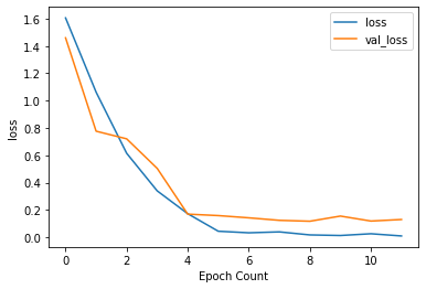
    56/56 - 6s - loss: 0.0102 - accuracy: 0.9994 - val_loss: 0.1306 - val_accuracy: 0.9663

We plot the history for accuracy and loss and see if there is overfitting.

def plot_graphs(history, string):
  plt.plot(history.history[string])
  plt.plot(history.history['val_'+string])
  plt.xlabel("Epoch Count")
  plt.ylabel(string)
  plt.legend([string, 'val_'+string])
  plt.show()
  
plot_graphs(history, "accuracy")
plot_graphs(history, "loss")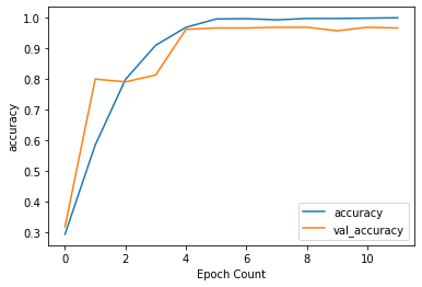

Finally, we call the method predict() to perform prediction on a sample text.

txt = ["Only bonds issued by the Russian government can be traded as part of a phased re-opening of the market. The exchange closed hours after Russian President Vladimir Putin sent thousands of troops into Ukraine on 24 February.Andrei Braginsky, a spokesman for the Moscow Exchange, said he hoped that trading in stocks would be able to start again soon. Technically everything is ready, and we are hoping this will resume in the near future, he said."]

seq = tokenizer.texts_to_sequences(txt)
padded = pad_sequences(seq, maxlen=max_length)
pred = model.predict(padded)
labels = ['sport', 'bussiness', 'politics', 'tech', 'entertainment'] 

print(pred)
print(np.argmax(pred))
print(labels[np.argmax(pred)-1])

    [[2.6411068e-04 2.1545513e-02 9.6170175e-01 7.2104726e-03 1.0733245e-03
      8.2047796e-03]]
    2
    bussiness

7. Conclusion

In this tutorial, we’ve build a text classification model with LSTM to predict the category of the BBC News articles. We examined two ways to import our data, using (1) GridDB and (2) With Statement. For large datasets, GridDB provides an excellent alternative to import data in your notebook as it is open-source and highly scalable. Download GridDB today!

If you have any questions about the blog, please create a Stack Overflow post here https://stackoverflow.com/questions/ask?tags=griddb .
Make sure that you use the “griddb” tag so our engineers can quickly reply to your questions.