Stroke Prediction using Machine Learning, Python, and GridDB

Stroke is a severe cerebrovascular disease caused by an interruption of blood flow from and to the brain. As a direct consequence of this interruption, the brain is not able to receive oxygen and nutrients for its correct functioning. The other way around, the brain is not able to drain and expulse through blood vessels all of its waste, like dead cells. In a question of minutes, the brain is in a critical condition as brain cells will imminently begin to die.

The American Stroke Association indicates that stroke is the fifth cause of death and disability in the United States. For this reason, stroke is considered a severe disease and has been the subject of extensive research, not only in the medical field but also in data science and machine learning studies. In this article, we propose a machine learning model to predict stroke diseases given patient records using Python and GridDB.

Setting up your environment

To accomplish the solution presented in this article, we begin by setting up the correct environment in your machine to correctly execute the presented code. Here are some of the requirements that need to be configured in your environment:

Windows 10. We are using Windows 10 as our main operating system.
GridDB. We use GridDB as our main database that stores the data used in the machine learning model.
Python 3.9. We use Python thanks Anaconda Navigator that allow deploying isolated working environments
Jupyter Notebook is used as our main computing platform to execute Python cells.
Microsoft Visual C++ 14.0 or greater. This is needed for JPype1 used by GridDB to execute commands on Jupyter Notebook.
Finally, we need to install any missing libraries that will be used in Jupyter Notebook. In our case, we were missing JPype1, scikit-plot, imblearn. Here is how we install missing libraries, thanks to pip command, in the Jupyter terminal:

  pip install imblearn   
  pip install scikit-plot   
  pip install JayDeBeApi JPype1==0.6.3  
  pip install pywaffle

Once we have successfully installed and configured our environment, we can step right into our dataset.

Introduction to the dataset

The dataset used in this article contains 5110 records of patients. Each patient has 12 columns each referring to a concrete attribute. Most of these attributes correspond to medical records or the results of clinical trials. Some of the key attributes are hypertension, heart diseases, average glucose levels in the blood, and body mass index (BMI). As we can observe from these first attributes, the dataset provides relevant data regarding the likelihood of patients suffering from stroke disease. It’s is easy to understand that a patient with high glucose levels and BMI, who has suffered from heart diseases and/or hypertension, is more likely to suffer from stroke. In fact, stroke is also an attribute in the dataset and indicates in each medical record if the patient suffered from a stroke disease or not.

The dataset is obtained from Kaggle and is available for download. The following table provides an extract of the dataset used in this article.

Importing the necessary libraries

In this article we will be using multiple python libraries, that we will organize according to their usage:

Libraries for linear algebra and data processing:

  import numpy as np 
  import pandas as pd

Libraries for plotting graphs

  import matplotlib.pyplot as plt
  import matplotlib.ticker as mtick
  import matplotlib.gridspec as grid_spec
  import seaborn as sns
  from imblearn.over_sampling import SMOTE
  import scikitplot as skplt

Libraries for building the model

  from sklearn.pipeline import Pipeline
  from sklearn.preprocessing import StandardScaler,LabelEncoder
  from sklearn.model_selection import train_test_split,cross_val_score
  
  from sklearn.metrics import classification_report, confusion_matrix
  from sklearn.metrics import accuracy_score, recall_score, roc_auc_score, precision_score, f1_score

Libraries for evaluating the model using different algorithms

from sklearn.linear_model import LinearRegression,LogisticRegression
  from sklearn.tree import DecisionTreeRegressor,DecisionTreeClassifier
  from sklearn.ensemble import RandomForestClassifier

Library for reading data from GridDB in Jupyter Notebook

import jaydebeapi

After we have successfully imported the required libraries, we begin by loading our dataset.

Loading the Dataset

In order to load the dataset we have two options that are described in more detail in the next paragraphs:

For the purpose of this article, we have already designed and loaded our data into a GridDB container. The article about using Pandas with GridDB can be useful if you want to write your data.

However, in this article, we do not read data from GridDB using Pandas, but we achieve this operation directly from the Jupyter Notebook, using the GridDB JDBC connector. The article on using GridDB in Jupyter can be very useful if more details are needed on this step. Here is the code to achieve this:

   def query_sensor(curs, table):
       curs.execute("select count(*) from "+table)
       return curs.fetchall()[0][0]
   
   conn = jaydebeapi.connect("com.toshiba.mwcloud.gs.sql.Driver", "jdbc:gs://239.0.0.1:41999/defaultCluster", ["admin", "admin"], "gridstore-jdbc-4.6.0.jar")
   curs = conn.cursor()
   curs.execute("select * from \"#tables\"")
   tables = []
   data = []
   
   for table in curs.fetchall():
       try:
           if table[1].split("_")[1].startswith("M"):
               tables.append(table[1])
               data.append(query_sensor(curs, table[1]))
       except:
           pass

You can also load the dataset using the CSV file downloaded from Kaggle. Make sure to place the file in the root directory of your Jupyter project, and it should be ready to be used:

   df = pd.read_csv('healthcare-dataset-stroke-data.csv')

For the purposes of this article, we will proceed with the data provided in the df variable.

Exploratory Data Analysis

Before we proceed to build our machine learning model, we must begin with an exploratory data analysis that will allow us to find any inconsistencies in our data, as well as overall visualization of the dataset.

First, we begin by checking for any null values in our dataset. This is achieved with the following lines of code:

df.isnull().sum()

This cell outputs the following results, indicating that we have 201 missing values for the BMI attribute:

id                     0
gender                 0
age                    0
hypertension           0
heart_disease          0
ever_married           0
work_type              0
Residence_type         0
avg_glucose_level      0
bmi                  201
smoking_status         0
stroke                 0
dtype: int64

In this case, we can simply opt for removing the missing values, but we will use a decision tree in order to predict the BMI values for the missing entries, a method described in a Kaggle notebook. This is achieved with the following code:

DT_bmi_pipe = Pipeline( steps=[ 
                               ('scale',StandardScaler()),
                               ('lr',DecisionTreeRegressor(random_state=42))
                              ])
X = df[['age','gender','bmi']].copy()
X.gender = X.gender.replace({'Male':0,'Female':1,'Other':-1}).astype(np.uint8)

Missing = X[X.bmi.isna()]
X = X[~X.bmi.isna()]
Y = X.pop('bmi')
DT_bmi_pipe.fit(X,Y)
predicted_bmi = pd.Series(DT_bmi_pipe.predict(Missing[['age','gender']]),index=Missing.index)
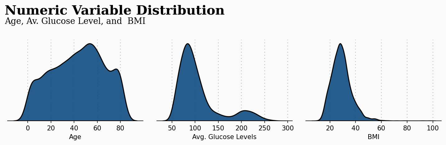
df.loc[Missing.index,'bmi'] = predicted_bmi

Now we have replaced all missing values, we can move to visualize our data. The first graph provides a numeric variable distribution of three key attributes that are age, average glucose levels, and BMI. This plot gives us a clear initial visualization of our data, being able to detect frequent age ranges, glucose levels, and BMIs. The code used to generate this plot is attached to the notebook in the public repository for this article.

The previous plot takes more importance when applied to our current study. The following plot makes a relation with the previous numeric attributes with the patient condition of suffering a stroke or not. This plot gives us great insights, and the code is also available in the GitHub repository.

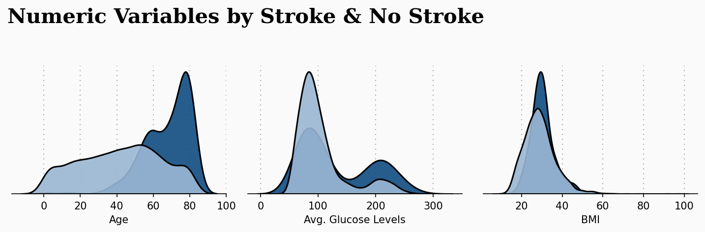
As we can observe, age seems to play a decisive factor in increasing the risk of a patient suffering from a stroke attack. We can observe that the older a patient, the increased the likelihood of suffering from stroke.

Machine Learning Model

In this section, we design and prepare our machine learning model. For this purpose, we begin by encoding the categorical variables present in our dataset. These include gender, residence type, and work type. We achieve this operation with the following code:

df['gender'] = df['gender'].replace({'Male':0,'Female':1,'Other':-1}).astype(np.uint8)
df['Residence_type'] = df['Residence_type'].replace({'Rural':0,'Urban':1}).astype(np.uint8)
df['work_type'] = df['work_type'].replace({'Private':0,'Self-employed':1,'Govt_job':2,'children':-1,'Never_worked':-2}).astype(np.uint8)

Now we have prepared our dataset, we will proceed to split our data into a training and testing data. Also, we need to make sure that the stoke attribute is not present in the dataset so we can correctly make the predictions. This is achieved thanks to the following code:

X = df[['gender','age','hypertension','heart_disease','work_type','avg_glucose_level','bmi']]y = df['stroke']
from sklearn.model_selection import train_test_split
X_train, X_test, y_train, y_test = train_test_split(X, y, train_size=0.3, random_state=42)

The dataset presented in this article is imbalanced. We have detected that the dataset is biased, so we have opted for SMOTE (Synthetic Minority Over-sampling Technique) to solve this issue. The following lines of code apply SMOTE over-sampling to our dataset, and result in a balanced dataset:

oversample = SMOTE()
X_train_resh, y_train_resh = oversample.fit_resample(X_train, y_train.ravel())

Model Evaluation

At this moment, we are ready to evaluate our model. In this example, we will use a random forest algorithm in order to evaluate the model that was designed in previous sections. In fact, we can use other classification models, like logistic regression, but we have noticed that the random forest obtains the highest accuracy. First, we begin by scaling our data in the pipeline and split it, thanks to the following lines of code:

rf_pipeline = Pipeline(steps = [('scale',StandardScaler()),('RF',RandomForestClassifier(random_state=42))])

To execute the algorithm, we use 10 fold cross validation:

print('Random Forest mean :',cross_val_score(rf_pipeline,X_train_resh,y_train_resh,cv=10,scoring='f1').mean())

The previous line of code outputs the following result:

Random Forest mean: 0.9342717632419655

As we can see, the random forest model was able to reach an accuracy of 93% in predicting patient records of suffering or not from stroke disease.

Conclusion

The combination of medical studies with machine learning and data science research can provide unprecedented insights for different diseases. In this article, we have explored the use of a machine learning model to predict the likelihood of medical patients suffering from stroke disease, a severe illness that affects the correct functioning of the human brain.

Reference

https://www.stroke.org/en/
https://github.com/almahdibakkali96/Stroke-Prediction-using-Machine-Learning-Python-and-GridDB-
https://www.kaggle.com/code/joshuaswords/predicting-a-stroke-shap-lime-explainer-eli5
https://www.kaggle.com/code/thomaskonstantin/analyzing-and-modeling-stroke-data/notebook

If you have any questions about the blog, please create a Stack Overflow post here https://stackoverflow.com/questions/ask?tags=griddb .
Make sure that you use the “griddb” tag so our engineers can quickly reply to your questions.

E-commerce Data Analysis using GridDB

Using SQL Batch Inserts with...

Analyzing Movies on IMDB using...

Building a Blog Voting Web...