
In this tutorial, we will explore the Heart Failure Prediction dataset which is publicly available on Kaggle. We will use GridDB to see how can we extract the data. Later, we will perform some Exploratory Data Analysis. Finally, we will build a Machine Learning Model for making future predictions. The outline of this tutorial is as follows:
- Setting up your environment
- Introduction to the dataset
- Importing the necessary libraries
- Loading the Dataset
- Exploratory Data Analysis
- Handling categorical variables
- Machine Learning Model
- Model Evaluation
- Conclusion
- References
You can read the Jupyter file here: https://github.com/griddbnet/Blogs/blob/main/Heart%20Failure%20Prediction.ipynb
1. Setting up your environment
The following tutorial is carried out in Jupyter Notebooks (Anaconda version 4.8.3) with Python version 3.8 on Windows 10 Operating system. Below mentioned packages need to be installed before the code execution:
The hyperlinks will direct you to the installation. Alternatively, if you are using a command line, simply type pip install package-name. Or in the case of Anaconda, conda install package-name also works.
While loading the dataset, this tutorial will cover two methods – Using GridDB as well as Using Pandas. To access GridDB using Python, the following packages also need to be installed beforehand:
- GridDB C-client
- SWIG (Simplified Wrapper and Interface Generator)
- GridDB Python Client
2. Introduction to the dataset
Cardiovascular disease is one of the leading causes of death worldwide. Therefore, if machine learning could help predict heart failure prediction, the contribution would be significant. The dataset used in this tutorial has been developed by Davide Chicco, Giuseppe Jurman of BMC Medical Informatics and Decision Making. It has been open-sourced and can be downloaded from Kaggle.
The data contains a total of 918 instances (or rows) with 12 attributes (or columns). Out of these 12 attributes, 5 are categorical and 7 are numerical in nature. Let’s now go ahead and import the necessary libraries.
3. Importing the necessary libraries
import numpy as np
import pandas as pd
import matplotlib.pyplot as plt
import seaborn as sns
from sklearn.model_selection import train_test_split
import plotly.graph_objects as go
import plotly.express as px
from sklearn.linear_model import LogisticRegression
from sklearn.metrics import classification_report
from sklearn.metrics import plot_confusion_matrix
If the installation was successful, the above cell should execute just fine without any error messages or warnings. However, if you do encounter an error –
- Recheck if the installation was successful. If not, execute
pip install package-nameagain. - Check if the version of the packages installed is compatible with your anaconda/system version.
4. Loading the dataset
4.1 Using GridDB
GridDB is a scalable, in-memory, No SQL database which makes it easier for you to store large amounts of data. Using GridDB’s python-client, we can now directly load our data as a pandas dataframe into the python environment. If you are new to GridDB, a tutorial on reading and writing to GridDB can be useful.
Assuming that you have already set up your database, we will now write the SQL query in python to load our dataset
import griddb_python as griddb

sql_statement = ('SELECT * FROM heart_failure_prediction')
heart_dataset = pd.read_sql_query(sql_statement, cont)
The cont variable has the container information where the data is stored.
4.2 Using Pandas
Alternatively, we can use the pandas read_csv() function. Note that both the methods would result in the same output as both loads the data in the form of a pandas dataframe.
heart_dataset = pd.read_csv('heart.csv')5. Exploratory Data Analysis
Let us first determine the shape of our dataset i.e the number of rows and number of columns
heart_dataset.shape(918, 12)
We will now display the first five rows of our data using the pandas head function to get a gist of how our data looks like.
heart_dataset.head()| Age | Sex | ChestPainType | RestingBP | Cholesterol | FastingBS | RestingECG | MaxHR | ExerciseAngina | Oldpeak | ST_Slope | HeartDisease | |
|---|---|---|---|---|---|---|---|---|---|---|---|---|
| 0 | 40 | M | ATA | 140 | 289 | 0 | Normal | 172 | N | 0.0 | Up | 0 |
| 1 | 49 | F | NAP | 160 | 180 | 0 | Normal | 156 | N | 1.0 | Flat | 1 |
| 2 | 37 | M | ATA | 130 | 283 | 0 | ST | 98 | N | 0.0 | Up | 0 |
| 3 | 48 | F | ASY | 138 | 214 | 0 | Normal | 108 | Y | 1.5 | Flat | 1 |
| 4 | 54 | M | NAP | 150 | 195 | 0 | Normal | 122 | N | 0.0 | Up | 0 |
Great! There is a mix of categorical and numerical values in this dataset. Note that we can not pass categorical variables directly to our machine learning model. We will have to encode them before model training. Let us go ahead and check the data types of our attributes.
heart_dataset.dtypesAge int64
Sex object
ChestPainType object
RestingBP int64
Cholesterol int64
FastingBS int64
RestingECG object
MaxHR int64
ExerciseAngina object
Oldpeak float64
ST_Slope object
HeartDisease int64
dtype: object
5 of the attributes have a data type of object which signifies that they are categorical in nature while the rest of them are either float or int which can be directly passed during the model training.
We will also get rid of the null values (if any) as they can produce an error during mathematical operations.
heart_dataset.isna().sum()Age 0
Sex 0
ChestPainType 0
RestingBP 0
Cholesterol 0
FastingBS 0
RestingECG 0
MaxHR 0
ExerciseAngina 0
Oldpeak 0
ST_Slope 0
HeartDisease 0
dtype: int64
Fortunately, we do not have any null values. We will now explore the categorical variables before moving on to the Machine Learning part.
categorical_cols= heart_dataset.select_dtypes(include=['object'])
categorical_cols.columns
Index(['Sex', 'ChestPainType', 'RestingECG', 'ExerciseAngina', 'ST_Slope'], dtype='object')
for cols in categorical_cols.columns:
    print(cols,'-', len(categorical_cols[cols].unique()),'Labels')
Sex - 2 Labels
ChestPainType - 4 Labels
RestingECG - 3 Labels
ExerciseAngina - 2 Labels
ST_Slope - 3 Labels
Since it is a single CSV file, it is better to split our dataset into train and test so that we can keep aside the test dataset for calculating the accuracy in later stages. We are using a 70-30 ratio for the train:test. The random_state variables ensure that these instances are picked randomly to minimize any bias or skewness.
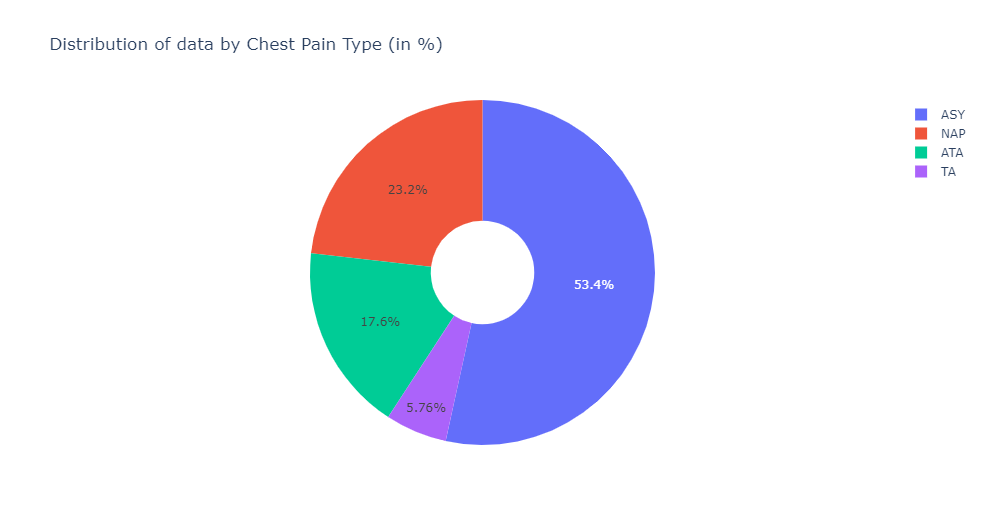
train, test = train_test_split(heart_dataset,test_size=0.3,random_state= 1234)labels = [x for x in train.ChestPainType.value_counts().index]
values = train.ChestPainType.value_counts()The distribution of data by Chest Pain Type —
fig = go.Figure(data=[go.Pie(labels=labels, values=values, hole=.3)])

fig.update_layout(
    title_text="Distribution of data by Chest Pain Type (in %)")
fig.update_traces()
fig.show()
Distribution of data by Gender which is further divided into whether a person has a heart disease or not —
fig=px.histogram(heart_dataset,
                 x="HeartDisease",
                 color="Sex",
                 hover_data=heart_dataset.columns,
                 title="Distribution of Heart Diseases by Gender",
                 barmode="group")
fig.show()
Try experimenting with other categorical variables using the histogram or pie function.
6. Handling categorical variables
We saw that the 2 attributes – Sex and ExerciseAngina among the 5 total categorical attributes are binary i.e. they only take two values. We can, therefore, manually encode these using 0 and 1. For the other values, we will use an encoding function.
train['Sex'] = np.where(train['Sex'] == "M", 0, 1)
train['ExerciseAngina'] = np.where(train['ExerciseAngina'] == "N", 0, 1)
test['Sex'] = np.where(test['Sex'] == "M", 0, 1)
test['ExerciseAngina'] = np.where(test['ExerciseAngina'] == "N", 0, 1)
<ipython-input-14-3d5da43d58db>:1: SettingWithCopyWarning:
A value is trying to be set on a copy of a slice from a DataFrame.
Try using .loc[row_indexer,col_indexer] = value instead
See the caveats in the documentation: https://pandas.pydata.org/pandas-docs/stable/user_guide/indexing.html#returning-a-view-versus-a-copy
<ipython-input-14-3d5da43d58db>:2: SettingWithCopyWarning:
A value is trying to be set on a copy of a slice from a DataFrame.
Try using .loc[row_indexer,col_indexer] = value instead
See the caveats in the documentation: https://pandas.pydata.org/pandas-docs/stable/user_guide/indexing.html#returning-a-view-versus-a-copy
<ipython-input-14-3d5da43d58db>:3: SettingWithCopyWarning:
A value is trying to be set on a copy of a slice from a DataFrame.
Try using .loc[row_indexer,col_indexer] = value instead
See the caveats in the documentation: https://pandas.pydata.org/pandas-docs/stable/user_guide/indexing.html#returning-a-view-versus-a-copy
<ipython-input-14-3d5da43d58db>:4: SettingWithCopyWarning:
A value is trying to be set on a copy of a slice from a DataFrame.
Try using .loc[row_indexer,col_indexer] = value instead
See the caveats in the documentation: https://pandas.pydata.org/pandas-docs/stable/user_guide/indexing.html#returning-a-view-versus-a-copy
train.head()| Age | Sex | ChestPainType | RestingBP | Cholesterol | FastingBS | RestingECG | MaxHR | ExerciseAngina | Oldpeak | ST_Slope | HeartDisease | |
|---|---|---|---|---|---|---|---|---|---|---|---|---|
| 578 | 57 | 0 | ASY | 156 | 173 | 0 | LVH | 119 | 1 | 3.0 | Down | 1 |
| 480 | 58 | 0 | ATA | 126 | 0 | 1 | Normal | 110 | 1 | 2.0 | Flat | 1 |
| 512 | 35 | 0 | NAP | 123 | 161 | 0 | ST | 153 | 0 | -0.1 | Up | 0 |
| 634 | 40 | 0 | TA | 140 | 199 | 0 | Normal | 178 | 1 | 1.4 | Up | 0 |
| 412 | 56 | 0 | ASY | 125 | 0 | 1 | Normal | 103 | 1 | 1.0 | Flat | 1 |
For attributes with 3 or more, we will use the pandas get_dummies function. It will create a new attribute per label. For instance, ChestPainType has 4 labels, therefore 4 new attributes will be created with a value of either 0 or 1.
train=pd.get_dummies(train)
test=pd.get_dummies(test)train.head()| Age | Sex | RestingBP | Cholesterol | FastingBS | MaxHR | ExerciseAngina | Oldpeak | HeartDisease | ChestPainType_ASY | ChestPainType_ATA | ChestPainType_NAP | ChestPainType_TA | RestingECG_LVH | RestingECG_Normal | RestingECG_ST | ST_Slope_Down | ST_Slope_Flat | ST_Slope_Up | |
|---|---|---|---|---|---|---|---|---|---|---|---|---|---|---|---|---|---|---|---|
| 578 | 57 | 0 | 156 | 173 | 0 | 119 | 1 | 3.0 | 1 | 1 | 0 | 0 | 0 | 1 | 0 | 0 | 1 | 0 | 0 |
| 480 | 58 | 0 | 126 | 0 | 1 | 110 | 1 | 2.0 | 1 | 0 | 1 | 0 | 0 | 0 | 1 | 0 | 0 | 1 | 0 |
| 512 | 35 | 0 | 123 | 161 | 0 | 153 | 0 | -0.1 | 0 | 0 | 0 | 1 | 0 | 0 | 0 | 1 | 0 | 0 | 1 |
| 634 | 40 | 0 | 140 | 199 | 0 | 178 | 1 | 1.4 | 0 | 0 | 0 | 0 | 1 | 0 | 1 | 0 | 0 | 0 | 1 |
| 412 | 56 | 0 | 125 | 0 | 1 | 103 | 1 | 1.0 | 1 | 1 | 0 | 0 | 0 | 0 | 1 | 0 | 0 | 1 | 0 |
test.head()| Age | Sex | RestingBP | Cholesterol | FastingBS | MaxHR | ExerciseAngina | Oldpeak | HeartDisease | ChestPainType_ASY | ChestPainType_ATA | ChestPainType_NAP | ChestPainType_TA | RestingECG_LVH | RestingECG_Normal | RestingECG_ST | ST_Slope_Down | ST_Slope_Flat | ST_Slope_Up | |
|---|---|---|---|---|---|---|---|---|---|---|---|---|---|---|---|---|---|---|---|
| 581 | 48 | 0 | 140 | 208 | 0 | 159 | 1 | 1.5 | 1 | 1 | 0 | 0 | 0 | 0 | 1 | 0 | 0 | 0 | 1 |
| 623 | 60 | 0 | 140 | 293 | 0 | 170 | 0 | 1.2 | 1 | 1 | 0 | 0 | 0 | 1 | 0 | 0 | 0 | 1 | 0 |
| 60 | 49 | 0 | 100 | 253 | 0 | 174 | 0 | 0.0 | 0 | 0 | 1 | 0 | 0 | 0 | 1 | 0 | 0 | 0 | 1 |
| 613 | 58 | 0 | 140 | 385 | 1 | 135 | 0 | 0.3 | 0 | 1 | 0 | 0 | 0 | 1 | 0 | 0 | 0 | 0 | 1 |
| 40 | 54 | 1 | 150 | 230 | 0 | 130 | 0 | 0.0 | 0 | 0 | 1 | 0 | 0 | 0 | 1 | 0 | 0 | 0 | 1 |
train.shape(642, 19)
test.shape(276, 19)
The total number of attributes have increased because of the encoding.
We will again divide our training and test sets into X and Y. X represents the set of independent variables/attributes which determine the outcome of the dependent variable, Y. In our case, the dependent variable or explanatory variable is HeartDisease.
x_train=train.drop(['HeartDisease'],1)
x_test=test.drop(['HeartDisease'],1)

y_train=train['HeartDisease']
y_test=test['HeartDisease']
print(x_train.shape)
print(x_test.shape)(642, 18)
(276, 18)
7. Machine Learning Model
Let us now build a Logistic Regression model with the following parameters —
max_iter=10000. Signifies maximum number of iterations taken for the solver to converge. The default choice is 100 iterations.penalty=l2. Signifies the norm used for penalty. Options include –None, l1, l2, and, elasticnet. The default is l2, so we do not have to provide it explicitly.
There are several parameters available for the function including class_weight, random_state, etc. Official documentation with usage and default parameters can be found here.
lr = LogisticRegression(max_iter=10000)
model1=lr.fit(x_train, y_train)
print("Train accuracy:",model1.score(x_train, y_train))Train accuracy: 0.8566978193146417
The training accuracy is approximately 85.6% which seems a decent start. Let us go ahead and make predictions for the test dataset.
8. Model Evaluation
print("Test accuracy:",model1.score(x_test,y_test))Test accuracy: 0.894927536231884
The test accuracy is nearly 89.5% which is higher than expected. Great! We can now store the predictions using the predict method on test dataset.
lrpred = lr.predict(x_test)8.1 Classification Report
The classification_report is one of the metrics in the scikit-learn library used for model evaluation. The function outputs the following:
Precision:Defined as True Positive/(True Positive+False Positive)Recall:Defined as True Positive/(True Positive+False Negative)F1 Score:The weighted harmonic mean of precision and recall. 1 signifies that both get equal weightage.Support:Number of occurences of each class in the ground truth.
print(classification_report(lrpred,y_test)) precision recall f1-score support
0 0.85 0.90 0.88 114
1 0.93 0.89 0.91 162
accuracy 0.89 276
macro avg 0.89 0.90 0.89 276
weighted avg 0.90 0.89 0.90 276
8.2 Confusion Matrix
Confusion Matrix is again one of the metrics used for evaluating your classifier. By definition, each entity (i,j) in the confusion matrix represents the observations that are actually in group i but classified under group j by your model. Explore more on what parameters can be customized for the confusion matrix here.
displr = plot_confusion_matrix(lr, x_test, y_test,cmap=plt.cm.OrRd , values_format='d')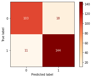
9. Conclusion
In this tutorial, we covered how can we use GriDB and Python to build a classifier for the Heart Failure Prediction Dataset. We covered two ways to access our data – Using GridDB and Pandas. GridDB is an efficient way when dealing with large amounts of data as it is highly scalable and open-source. Install GridDB today!
10. References
- https://www.kaggle.com/fedesoriano/heart-failure-prediction
- https://www.kaggle.com/sisharaneranjana/machine-learning-to-the-fore-to-save-lives
- https://www.kaggle.com/durgancegaur/a-guide-to-any-classification-problem
If you have any questions about the blog, please create a Stack Overflow post here https://stackoverflow.com/questions/ask?tags=griddb .
Make sure that you use the “griddb” tag so our engineers can quickly reply to your questions.