
Economic indicators have been used in numerous studies to forecast stock prices using well-known statistical methods. The rising power of computers since *2010 has resulted in the development of new methods of machine learning. To discover whether those algorithms can predict the stock market using a variety of mathematical and statistical methods would be interesting. The purpose of this article is to model the monthly price of the S&P 500 index based on U.S. economic indicators using GridDB to extract the data, followed by performing the statistical tests and finally building the machine learning model.
The outline of the tutorial is as follows:
- Prerequisites and Environment setup
- Dataset overview
- Importing required libraries
- Loading the dataset
- Exploratory Data Analysis & Feature Selection
- Building and Training a Machine Learning Model
- Conclusion
Prerequisites and Environment setup
This tutorial is carried out in Anaconda Navigator (Python version – 3.8.3) on Windows Operating System. The following packages need to be installed before you continue with the tutorial –
-
Pandas
-
NumPy
-
Scikit-learn
-
Matplotlib
-
Statsmodels
-
griddb_python
You can install these packages in Conda’s virtual environment using conda install package-name. In case you are using Python directly via terminal/command prompt, pip install package-name will do the work.
GridDB installation
While loading the dataset, this tutorial will cover two methods – Using GridDB as well as Using Pandas. To access GridDB using Python, the following packages also need to be installed beforehand:
- GridDB C-client
- SWIG (Simplified Wrapper and Interface Generator)
- GridDB Python Client
1. Dataset Overview
The indicators that are recognised to have the most significant impact on stock market return in general and on S&P 500 in particular can be attributed to the following categories: general macroeconomic indicators, labour market indicators (unemployment rate and jobs reports), real estate indicators, credit market indicators, monetary supply indicators, consumer (household) financial behaviour indicators and commodity market indicators.
The S&P 500 index close price was modelling in this paper. The study used a python programming language with many libraries in Google Colab environment. The analysis period between 1970-01-01 / 2018-04-01, and both S&P 500 index close price and U.S economic indicators data frequency are month.
Feature Description:
1) SP500 – Price of S&P 500 at respective month (Units: U.S. Dollars)
2) INTDSRUSM193N – Interest Rates, Discount Rate for United States (Units: Percent per Annum)
3) BUSLOANS – Commercial and Industrial Loans, All Commercial Banks (Units: Billions of U.S. Dollars)
4) MPRIME – Bank Prime Loan Rate (Units: Percent)
5) FEDFUNDS – Federal Funds Effective Rate (The federal funds rate is the interest rate at which depository institutions trade federal funds with each other overnight.) (Units: Percent)
6) CURRCIR – Currency in Circulation (Units: Billions of Dollars)
7) PSAVERT – Personal Saving Rate (Personal saving as a percentage of disposable personal income (DPI), frequently referred to as “the personal saving rate,” is calculated as the ratio of personal saving to DPI.)(Units: Percent)
8) PERMIT – New Privately-Owned Housing Units Authorized in Permit-Issuing Places: Total Units (Units: Billions of Dollars)
9) INDPRO – Industrial Production: Total Index (The Industrial Production Index (INDPRO) is an economic indicator that measures real output for all facilities located in the United States manufacturing, mining, and electric, and gas utilities) (Units: Index 2017=100)
10) PMSAVE – Personal Saving (Units: Billions of Dollars)
11) DAUTOSAAR – Motor Vehicle Retail Sales: Domestic Autos (Units: Millions of Units)
12) UNEMPLOY – Unemployment Level (Units: Thousands of Persons)
13) CPIAUCSL – Consumer Price Index for All Urban Consumers: All Items in U.S. City Average (Units: Index 1982-1984=100)
The dataset is available publicly and can be downloaded from finance.yahoo.com and fred.stlouisfed.org website. The obtained data were combined into one data set, which was checked for missing values.
2. Importing Required Libraries
import griddb_python as griddb

import numpy as np
import pandas as pd
import matplotlib.pyplot as plt
import datetime

import statsmodels.api as sm
from statsmodels.stats.outliers_influence import variance_inflation_factor

from sklearn.model_selection import train_test_split
from sklearn.linear_model import LinearRegression
from sklearn.ensemble import RandomForestRegressor
from sklearn.metrics import r2_score
from sklearn.metrics import mean_squared_error

import warnings
warnings.filterwarnings('ignore')
%matplotlib inline
3. Loading the Dataset
Let’s proceed and load the dataset into our notebook.
3.a Using GridDB
Toshiba GridDB™ is a highly scalable NoSQL database best suited for IoT and Big Data. The foundation of GridDB’s principles is based upon offering a versatile data store that is optimized for IoT, provides high scalability, tuned for high performance, and ensures high reliability.
To store large amounts of data, a CSV file can be cumbersome. GridDB serves as a perfect alternative as it in open-source and a highly scalable database. GridDB is a scalable, in-memory, No SQL database which makes it easier for you to store large amounts of data. If you are new to GridDB, a tutorial on reading and writing to GridDB can be useful.
Assuming that you have already set up your database, we will now write the SQL query in python to load our dataset.
sql_statement = ('SELECT * FROM us_economic_data')
dataset = pd.read_sql_query(sql_statement, cont)
Note that the cont variable has the container information where our data is stored. Replace the credit_card_dataset with the name of your container. More info can be found in this tutorial reading and writing to GridDB.
When it comes to IoT and Big Data use cases, GridDB clearly stands out among other databases in the Relational and NoSQL space. Overall, GridDB offers multiple reliability features for mission-critical applications that require high availability and data retention.
3.b Using Pandas
We can also use Pandas’ read_csv function to load our data. Both of the above methods will lead to the same output as the data is loaded in the form of a pandas dataframe using either of the methods.
us_economic_data = pd.read_csv('us_economic_data.csv')4. Exploratory Data Analysis & Feature Selection
Once the dataset is loaded, let us now explore the dataset. We’ll print the first 10 rows of this dataset using head() function.
us_economic_data.head()df = us_economic_data# Changing the column name and then setting the date as an index od the dataframe
df.rename(columns = {'Unnamed: 0':'date'}, inplace = True)
df['date'] = pd.to_datetime(df['date'])
df = df.set_index('date')df.head()We performed Augmented Dickey-Fuller to determine if S&P 500 close prices is stationary. Later, we made visualization of the data between the closing price and each independent variable to determine if there is a linear relationship between the variables and thus to select only those variables that it has.
After, we checked whether the independent variables correlated with each other using the VIF test. Finally, because the indicators are measured in different scales, the data were normalized using z score criteria to produce accurate and reliable mode
def tsplot(y, figsize=(12, 7), syle='bmh'):
if not isinstance(y, pd.Series):
y = pd.Series(y)
with plt.style.context(style='bmh'):
fig = plt.figure(figsize=figsize)
layout = (2,1)
ts_ax = plt.subplot2grid(layout, (0,0), colspan=2)
y.plot(ax=ts_ax)
p_value = sm.tsa.stattools.adfuller(y)[1]
ts_ax.set_title('Time Series Analysis Plotsn Dickey-Fuller: p={0:.5f}'.format(p_value))
plt.tight_layout()
tsplot(df['SP500'])
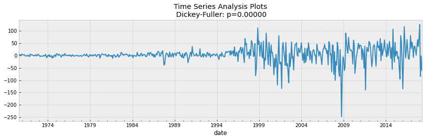
data_diff = df['SP500'] - df['SP500'].shift(1)
tsplot(data_diff[1:])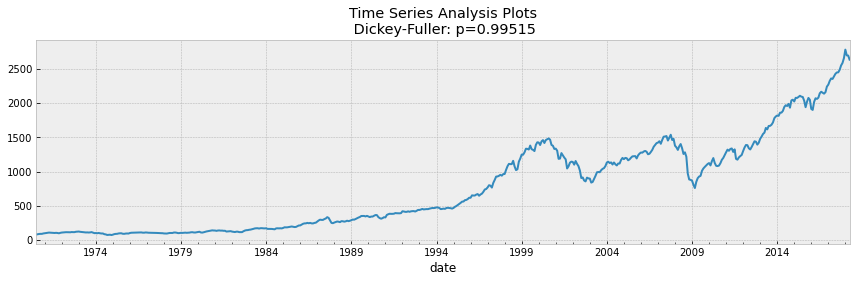
If we take 5% as the confidence level in our hypothesis of Dickey Fuller test, we can see that pvalue is much greater than 0.05 so the S&P 500 is not stationary.
To make the data stationary, it was necessary to create a new dependent variable, which was calculated from the current monthly price minus the previous month’s price. In this case, the tests mentioned earlier were recalculated and the data were found to be stationary since pvalue comes out to be 0.
The next step is to find if independent variables did not correlate with each other. The VIF test was chosen for this purpose. Variance Inflating factor (VIF) is used to test the presence of multicollinearity in a regression model.
df.columnsIndex(['SP500', 'INTDSRUSM193N', 'BUSLOANS', 'MPRIME', 'FEDFUNDS', 'CURRCIR',
'PSAVERT', 'PMSAVE', 'DAUTOSAAR', 'UNEMPLOY', 'INDPRO', 'PERMIT',
'CPIAUCSL'],
dtype='object')
# the independent variables set
X = df[['INTDSRUSM193N', 'BUSLOANS', 'MPRIME', 'FEDFUNDS', 'CURRCIR',
       'PSAVERT', 'PMSAVE', 'DAUTOSAAR', 'UNEMPLOY', 'INDPRO', 'PERMIT',
       'CPIAUCSL']]

# VIF dataframe
vif_data = pd.DataFrame()
vif_data["feature"] = X.columns

# calculating VIF for each feature
vif_data["VIF"] = [variance_inflation_factor(X.values, i)
                          for i in range(len(X.columns))]

print(vif_data)
feature VIF
0 INTDSRUSM193N 130.622837
1 BUSLOANS 147.284028
2 MPRIME 399.916868
3 FEDFUNDS 145.507021
4 CURRCIR 112.882897
5 PSAVERT 63.436200
6 PMSAVE 68.862740
7 DAUTOSAAR 60.502647
8 UNEMPLOY 54.757359
9 INDPRO 464.500794
10 PERMIT 34.696174
11 CPIAUCSL 897.072035
From the table it can be seen that the VIF test values for each variable are well above 10. In this case, the indicator with the highest VIF value is removed and the whole set is recalculated. This is done as long as all variables with values less than 10 remain.
# the independent variables set
X = df[[  'FEDFUNDS', 'CURRCIR','PSAVERT', 'PERMIT',]]

# VIF dataframe
vif_data = pd.DataFrame()
vif_data["feature"] = X.columns

# calculating VIF for each feature
vif_data["VIF"] = [variance_inflation_factor(X.values, i)
                          for i in range(len(X.columns))]

print(vif_data)
feature VIF
0 FEDFUNDS 5.228717
1 CURRCIR 2.532886
2 PSAVERT 8.150866
3 PERMIT 7.039288
We found that 11 of them did not meet the linear regression rule that the data should be linear.
The last thing in our second stage was to take those 3 indicators together with S&P 500 index price data and normalized them by z score criteria.
df_new = df[['SP500','FEDFUNDS','CURRCIR','PSAVERT','PERMIT']]df_z_scaled = df_new.copy()
# apply normalization techniques
for column in df_z_scaled.columns:
df_z_scaled[column] = (df_z_scaled[column] -
df_z_scaled[column].mean()) / df_z_scaled[column].std()
# view normalized data
df_z_scaled.head()| SP500 | FEDFUNDS | CURRCIR | PSAVERT | PERMIT | |
|---|---|---|---|---|---|
| date | |||||
| 1970-07-01 | -1.019219 | 0.500923 | -1.065075 | 1.792466 | -0.165538 |
| 1970-08-01 | -1.015924 | 0.351568 | -1.064918 | 1.758546 | 0.002858 |
| 1970-09-01 | -1.008946 | 0.268030 | -1.064531 | 1.588943 | 0.079839 |
| 1970-10-01 | -1.006266 | 0.245247 | -1.064222 | 1.656784 | 0.411821 |
| 1970-11-01 | -1.006401 | 0.093359 | -1.062341 | 1.826387 | 0.262670 |
5. Machine Learning Model Building
Now, let’s proceed to building and evaluating machine learning models on our credit card dataset. We’ll first create features and labels for our model and split them into train and test samples. Test size has been kept as 20% of the total dataset size.
features = df_z_scaled.drop(columns = ['SP500'], axis = 1)
labels = df_z_scaled[['SP500']]

X_train, X_test, y_train, y_test = train_test_split(features, labels, test_size = 0.2, random_state = 0)
print(f"Shape of training data: {X_train.shape}")
print(f"Shape of the training target data: {y_train.shape}")
print(f"Shape of test data: {X_test.shape}")
print(f"Shape of the test target data: {y_test.shape}")Shape of training data: (459, 4)
Shape of the training target data: (459, 1)
Shape of test data: (115, 4)
Shape of the test target data: (115, 1)
We started the third stage of the study by constructing a statistical linear regression model, which is our baseline.
regr = LinearRegression()

regr.fit(X_train, y_train)
print(regr.score(X_test, y_test))
0.9351836569209164
coefficients = pd.concat([pd.DataFrame(X.columns),pd.DataFrame(np.transpose(regr.coef_))], axis = 1)
coefficients| 0 | 0 | |
|---|---|---|
| 0 | FEDFUNDS | 0.083735 |
| 1 | CURRCIR | 1.003270 |
| 2 | PSAVERT | -0.087568 |
| 3 | PERMIT | 0.116120 |
Currency in Circulation has the highest coefficient which means highest impact to model.
After the model has been fit on our training data, we can proceed to predicting for our test set in order to evaluate the model performance. Lets store our predictions in predicted.
Evaluation Metric: 1) Coefficient of determination (R^2). This is the most important indicator of model confidence in the data, which is mandatory in all descriptions of regression models.
2) Mean square error (MSE). This value measures the root mean square error between actual and predicted values.
y_pred = regr.predict(X_test)
mse = mean_squared_error(y_test, y_pred)
print("MSE: ", mse)
print("RMSE: ", mse*(1/2.0))

r2 = r2_score(y_test, y_pred)
print('r2 score for Random Forest model is', r2)
MSE: 0.06275016232171571
RMSE: 0.031375081160857854
r2 score for Random Forest model is 0.9351836569209164
Random forest regression is a tree ensemble learning technique. Prediction based on the trees is more accurate because it takes into account many predictions. This is because of the average value used. These algorithms are more stable because any changes in dataset can impact one tree but not the forest of trees.
rfr = RandomForestRegressor()

rfr.fit(X_train, y_train)

score = rfr.score(X_train, y_train)
print("R-squared:", score)
R-squared: 0.9993703842202256
ypred = rfr.predict(X_test)

mse = mean_squared_error(y_test, ypred)
print("MSE: ", mse)
print("RMSE: ", mse*(1/2.0))

r2 = r2_score(y_test, ypred)
print('r2 score for Random Forest model is', r2)
MSE: 0.0031918233911353254
RMSE: 0.0015959116955676627
r2 score for Random Forest model is 0.9967030791266005
plt.figure(figsize=(5,5))
plt.scatter(y_test['SP500'].values, ypred, c='crimson')


p1 = max(max(ypred), max(y_test['SP500'].values))
p2 = min(min(ypred), min(y_test['SP500'].values))
plt.plot([p1, p2], [p1, p2], 'b-')
plt.xlabel('True Values', fontsize=15)
plt.ylabel('Predictions', fontsize=15)
plt.axis('equal')
plt.show()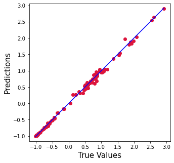
Comparison between baseline and Random Forest Model
The ML Random Forest model was found to be the better machine learning model because it provided highest R2 and lowest error rate. The statistical linear regression model was improved by 6 % and the error rate was reduced 20 times.
6. Conclusion
In this tutorial we identified 13 indicators that can have the most significant impact on stock markets and S&P 500 index in particular. We examined two ways to import our data, ussing (1) GridDB and (2) Pandas. For large datasets, GridDB provides an excellent alternative to import data in your notebook as it is open-source and highly scalable. Download GridDB today!